MOSFET DC Analysis and Q-Point

Recommended resources

The freely available resources this lesson will direct you to.

Introduction

In our last lesson, we focused on the fundamental tools for MOSFET analysis: the I-V equations for the triode and saturation regions and the "assume and verify" strategy. Today, we will use those tools to analyze the complete DC state of single-transistor circuits. Your learning goal is to determine the DC operating point, or Quiescent Point (Q-point), for various common MOSFET biasing configurations.

The Q-point represents the DC voltages and currents in the circuit when no input signal is applied. Establishing the correct Q-point is the most critical step in designing an amplifier, as it ensures the transistor is primed to operate in the desired region—typically saturation—for linear amplification. This lesson forms the analytical foundation for the amplifier circuits we will study in the next module.

What is the DC Operating Point (Q-point)?

Before a MOSFET can amplify a small AC signal, it must be set up with specific DC operating conditions. This process is called biasing. The resulting DC drain current ( $I_{D Q}$ ) and drain-to-source voltage ( $V_{D S Q}$ ) define the transistor's Q-point. Let's start by understanding why this is so crucial.

MOSFET Biasing : Enhancement Type MOSFET Biasing Explained

The video "MOSFET Biasing" from the ALL ABOUT ELECTRONICS channel provides an excellent conceptual overview of why we bias transistors.

Please watch the segment from the beginning. Focus on the explanation of why the MOSFET must be biased in the saturation region to function as an amplifier. The instructor uses the transistor's transfer characteristic to show that this region offers the most linear amplification.

As the video explained, the goal of biasing is to place the Q-point in the saturation region, where the drain current is strongly controlled by $V_{GS}$ and is relatively independent of $V_{D S}$ . This allows the transistor to act as a voltage-controlled current source, which is the basis of amplification.

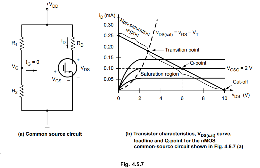
The DC Load Line: A Graphical View

We can visualize the Q-point graphically. For a typical common-source amplifier, Kirchhoff's Voltage Law (KVL) around the output loop (from the power supply $V_{D D}$ through the drain resistor $R_{D}$ and the MOSFET to ground) gives us an equation that relates $I_{D}$ and $V_{D S}$ :

V_{D D} = I_{D} R_{D} + V_{D S}

Rearranging this gives the equation for a straight line on the MOSFET's output characteristic graph:

I_{D} = - \frac{1}{R _{D}} V_{D S} + \frac{V _{D D}}{R _{D}}

This line is called the DC Load Line. It represents all possible combinations of $I_{D}$ and $V_{D S}$ that are permitted by the external circuit (i.e., by $R_{D}$ and $V_{D D}$ ). The actual operating point must lie on this line.

The Q-point is the specific point on the load line where the transistor's own physics (represented by its characteristic curve for a given $V_{GS Q}$ ) intersects with the constraints of the external circuit (represented by the load line).

The diagram on the left shows a common-source circuit with voltage divider biasing. The graph on the right shows its output characteristics. The straight line is the DC load line, and its intersection with the curve for $V_{GSQ} = 2V$ determines the circuit's Q-point, ($I_{DQ}, V_{DSQ}$).

A Systematic Approach to DC Analysis

While the graphical method is intuitive, circuit analysis is performed mathematically. In the previous lesson, you practiced the "assume and verify" method. We will now formalize this into a robust, five-step procedure that you can apply systematically to any DC MOSFET circuit—a crucial skill for your exams.

4.3 MOSFET Circuits at DC

This document from the University of Kansas outlines a clear, step-by-step methodology for DC analysis.

Please read the first part of the document, which details the five steps: <span data-type="resource_reading_textrange" data-resource-subitem-id="ebb1bbf4" data-range-start="1. ASSUME an operating mode" data-range-end="start completely over!">The 5-step process. Pay close attention to the ENFORCE and CHECK steps for each operating region, as this is the core of the method.

To summarize the resource, the five steps are:

ASSUME: Assume an operating region for the MOSFET (usually saturation for amplifiers).
ENFORCE: Use the I-V equation corresponding to the assumed region in your circuit analysis.
ANALYZE: Use KVL, KCL, and the enforced I-V equation to solve for the unknown currents and voltages ( $I_{D}$ , $V_{GS}$ , $V_{D S}$ ).
CHECK: Verify that the calculated voltages satisfy the inequality conditions for the assumed region (e.g., for saturation, check if $V_{D S} \geq V_{GS} - V_{t}$ ).
MODIFY: If the check fails, your assumption was wrong. You must start over with a new assumption (e.g., triode region) and re-analyze the circuit.

Analysis of Common Biasing Circuits

Let's now apply this five-step method to analyze some standard biasing circuits.

1. Voltage Divider Biasing

This is one of the most common and practical biasing schemes. You've already seen it in the previous lesson's examples. It uses a voltage divider to set the DC gate voltage, and a source resistor ( $R_{S}$ ) to provide stability.

Let's walk through a complete analysis of a typical voltage-divider biased circuit.

EE 203, 64- MOSFET: DC Analysis Example 1

This video, "MOSFET: DC Analysis Example 1" by Wessam Mesbah, provides a clear, step-by-step numerical solution for a voltage divider biased circuit.

Follow the instructor's application of our five-step method: Preparation: First, watch how the circuit is redrawn and the gate voltage V_G is calculated using the voltage divider rule at the beginning. This is always the first step for this configuration. Assume & Enforce: The instructor assumes saturation and writes the KVL equation for the gate-source loop. He then enforces the saturation I-V equation, substituting it into the KVL equation to get a single quadratic equation in terms of V_{GS}. Analyze: Next, he solves the quadratic equation. Note that it yields two solutions for V_{GS}. He correctly discards the one that is physically impossible (V_{GS} < V_t), as the transistor would be in cut-off. With the valid V_{GSQ}, he calculates the drain current I_{DQ}. Check: This is the final, crucial step. He applies KVL to the drain-source loop to find V_{DSQ}. Then, he checks the saturation condition (V_{DS} \ge V_{GS} - V_t). Since the condition holds, the initial assumption was correct, and the analysis is complete.

The process demonstrated in the video is the complete blueprint for analyzing voltage-divider bias circuits.

2. Constant-Current Source Biasing

In integrated circuits (ICs), resistors take up a lot of chip area. A more efficient and stable way to bias a MOSFET is to use a constant-current source in place of the source resistor $R_{S}$ . This forces the drain current $I_{D}$ to be a fixed, known value, $I_{Q}$ .

Circuit (a) shows an NMOS amplifier biased with an ideal current source $I_Q$. Circuit (b) shows the equivalent DC circuit used for analysis.

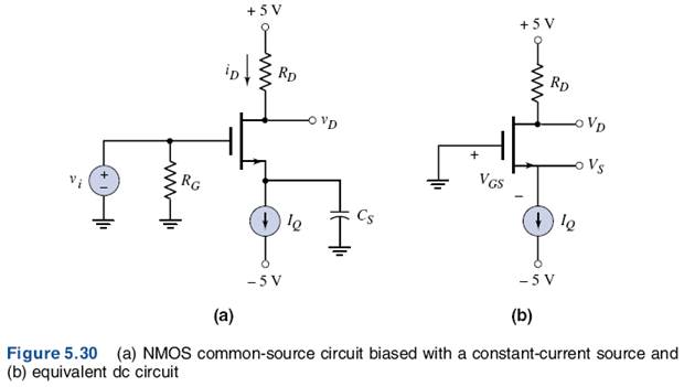
Analysis of this circuit is often more straightforward:

Assume the transistor is in saturation.
Enforce the known drain current: $I_{D Q} = I_{Q}$ .
Analyze to find the voltages. Use the saturation I-V equation to find the required $V_{GS Q}$ : $I_{D Q} = I_{Q} = \frac{1}{2} k_{n} (V_{GS Q} - V_{t})^{2} ⟹ Solve for V_{GS Q}$ Then, find $V_{S}$ from $V_{GS Q}$ (since $V_{G}$ is often known, e.g., grounded) and $V_{D}$ from KVL in the output loop.
Check if the saturation condition ( $V_{D S Q} \geq V_{GS Q} - V_{t}$ ) is met.

This biasing method provides excellent stability against variations in temperature and device parameters. In later lessons, you will learn how these "constant-current sources" are built using other transistors, forming circuits known as current mirrors.

When the Assumption Fails

What happens if the "CHECK" step fails? This means your initial assumption was incorrect, and you must re-do the analysis using the equations for the correct region, which is usually the triode region. The following reading walks through exactly such a scenario.

4.3 MOSFET Circuits at DC

This example from the same University of Kansas notes demonstrates the full "Assume-Check-Modify" cycle.

Please read through the PMOS example. Follow the logic carefully: The analysis begins by assuming saturation. All the DC values are calculated based on this assumption. During the CHECK step, it is found that V_{SD} < V_{SG} - |V_{tp}|, which violates the saturation condition for a PMOS device. The text correctly states: "our ASSUMPTION was incorrect!". The analysis is restarted from scratch, this time assuming the triode region. The triode I-V equation is enforced. New values are calculated, and the CHECK step for the triode region (V_{SD} < V_{SG} - |V_{tp}|) is performed. This time it passes, confirming the triode assumption is correct.

Mastering this full cycle is vital. On an exam, you may well be given a circuit that is not in saturation, and demonstrating your ability to correctly identify and analyze it will be critical.

Conclusion

In this lesson, we formalized the process of DC analysis for MOSFET circuits. You have learned how to find the all-important Q-point, which sets the stage for a transistor's behavior as an amplifier.

Here are the key takeaways:

The DC Operating Point (Q-point), defined by $(I_{D Q}, V_{D S Q})$ , is the steady-state condition of a transistor with no AC signal. Proper biasing aims to place this point in the saturation region for amplification.
The DC Load Line provides a graphical method to visualize the Q-point as the intersection of the external circuit's constraints and the transistor's characteristics.
A robust, five-step method (Assume, Enforce, Analyze, Check, Modify) provides a reliable algorithm for solving any DC MOSFET circuit problem.
You are now familiar with the analysis of several key biasing topologies, including voltage divider bias and constant-current source bias.

In our next lesson, we will build upon this foundation by exploring a common technique in modern IC design: using another transistor as the load resistor ( $R_{D}$ ). This is known as using an active load, and its analysis directly uses the Q-point skills you have developed today.