Down Payments & Interest Rates: Impact on Cash Flow & Returns

Hello! Welcome back to our course on real estate investment analysis.

In our last few lessons, we built a solid foundation for analyzing a single deal. We learned to calculate pre-tax cash flow, cash-on-cash (CoC) return, and equity buildup, each for a specific set of financing terms. However, real-world deal analysis is rarely static. The financing you secure can dramatically alter an investment's performance.

Today's lesson is about moving from static calculation to dynamic analysis. We will explore how changing two of the most critical financing variables—the down payment amount and the interest rate—impacts your cash flow and returns. This process, known as sensitivity analysis, is fundamental to understanding the risks and opportunities of a leveraged real estate investment.

By the end of this 60-minute lesson, you will be able to analyze and quantify the trade-offs involved in different financing structures, allowing you to make more informed investment decisions.

1. The Core Trade-Off: Leverage, Cash Flow, and Returns

The amount of money you put down on a property is one of the most significant decisions you'll make. It creates a fundamental trade-off between your monthly cash flow and the magnification of your returns through leverage.

• Higher Down Payment: You borrow less, which means your monthly mortgage payment is lower. This directly results in higher pre-tax cash flow. However, you've invested more of your own capital, which typically leads to a lower cash-on-cash (CoC) return.
• Lower Down Payment: You borrow more (higher leverage). Your mortgage payments are higher, leading to lower pre-tax cash flow. But since your initial cash investment is smaller, the CoC return can be significantly higher, magnifying your gains (and potential losses).

As the article highlights, with leverage, your return is calculated on a smaller base of your own capital, while the profit is generated from the total value of the asset. This is the "magic" of leverage that amplifies returns.

2. The Impact of Interest Rates

The effect of interest rates is more straightforward but no less critical. The interest rate is the direct cost of the leverage you employ.

• A higher interest rate increases your monthly debt service, which directly reduces your pre-tax cash flow and, consequently, your CoC return.
• A lower interest rate does the opposite, leaving more money in your pocket each month and boosting your returns.

This becomes especially important when considering variable-rate mortgages, which are common in Spain and are typically tied to the Euríbor. A sharp rise in the Euríbor can turn a cash-flowing property into a liability.

The Parlantia article you just read discusses this risk under the heading "El lado oscuro: cómo el apalancamiento amplifica el riesgo," specifically in the subsection "Subida de tipos de interés" (Section 2). It provides a timely example of how the Euríbor hikes in 2022-2023 impacted investors. To mitigate this, many investors prefer fixed-rate mortgages, especially in an uncertain rate environment, a strategy mentioned in the article's "Estrategias para maximizar rentabilidad" section (Section 3).

3. Visualizing the Impact: Sensitivity Analysis

How can we systematically analyze these trade-offs? The answer is sensitivity analysis, a modeling technique used to determine how different values of an independent variable (like interest rate) will impact a particular dependent variable (like cash flow).

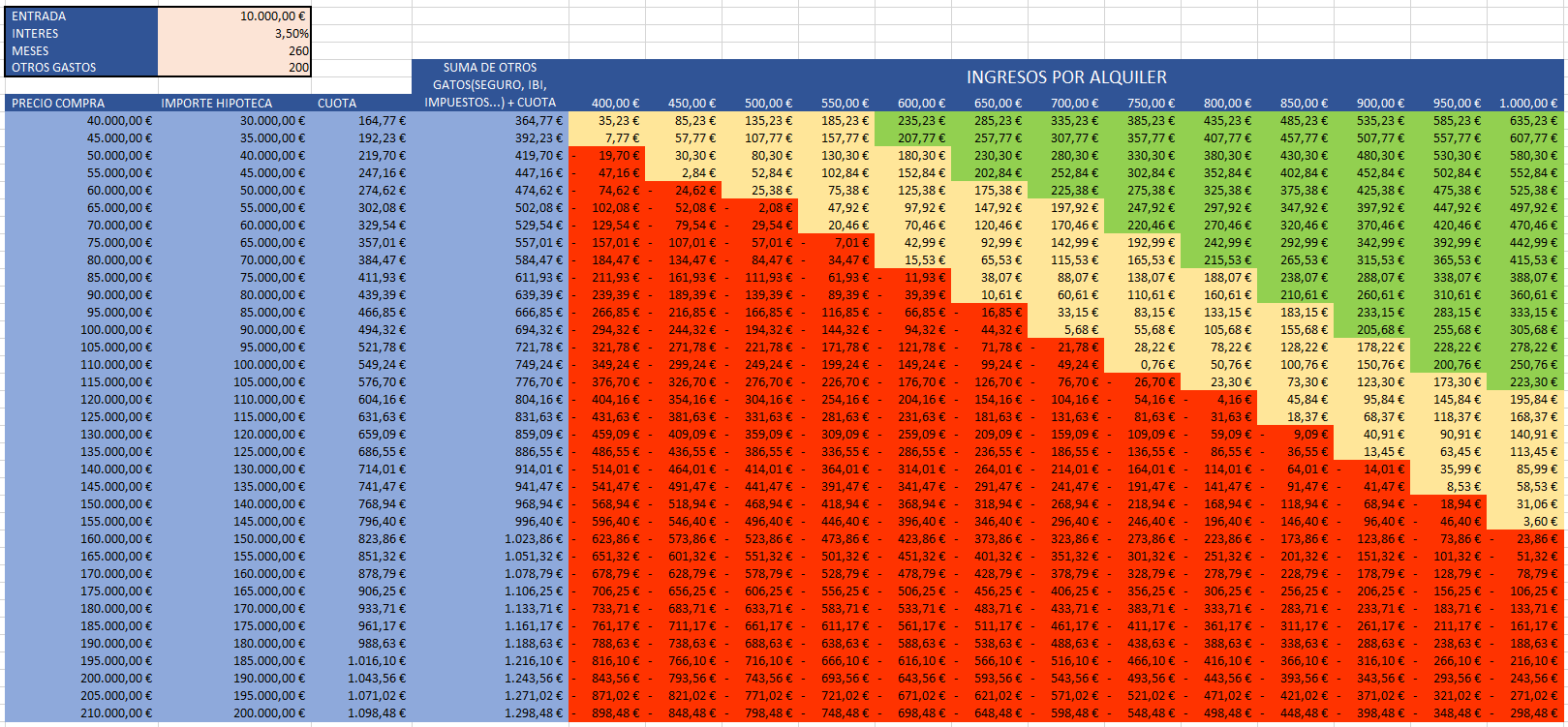
A common way to perform a two-variable sensitivity analysis is to create a data table or matrix. For our purposes, we can set up a grid:

• The rows could represent different down payment percentages.
• The columns could represent different annual interest rates.
• The value in each cell of the grid would be the resulting metric we want to analyze, such as Pre-Tax Cash Flow or CoC Return.

This gives you an immediate, comprehensive picture of the investment's financial landscape under various scenarios.

The resulting table allows you to see at a glance how robust your investment is. For example, you can identify the "break-even" interest rate at which your cash flow turns negative for a given down payment.

4. Modeling Sensitivity Analysis in Python

Now, let's translate this concept into code. Your background in software engineering makes this a natural fit. We'll use the numpy-financial library for our mortgage calculations and pandas to create a clean, readable data table.

We will write a script that generates two sensitivity tables for a given property:

1. Pre-Tax Cash Flow vs. Down Payment & Interest Rate
2. Cash-on-Cash Return vs. Down Payment & Interest Rate

The script will loop through each combination of financing terms and calculate the metrics, populating a pandas DataFrame that mirrors the tables we've discussed.

Here is the Python code to perform this analysis. It brings together concepts from our previous lessons (NOI, debt service, CoC return) into a single, powerful script.

# Ensure you have the necessary libraries installed:
# pip install numpy-financial pandas

import numpy_financial as npf
import pandas as pd

# --- Property & Investment Assumptions ---
PURCHASE_PRICE = 200000  # €
CLOSING_COSTS_PCT = 0.10 # 10% for ITP, notary, etc. in Spain
NET_OPERATING_INCOME = 9300 # € per year (from previous lessons)
LOAN_TERM_YEARS = 30

# --- Sensitivity Analysis Parameters ---
DOWN_PAYMENT_RATES = [0.20, 0.25, 0.30, 0.35]
ANNUAL_INTEREST_RATES = [0.025, 0.03, 0.035, 0.04, 0.045]

def analyze_financing_sensitivity(price, noi, term, dp_rates, interest_rates):
    """
    Performs a sensitivity analysis on cash flow and CoC return
    based on down payment and interest rates.
    """
    # Initialize empty DataFrames to store results
    cash_flow_df = pd.DataFrame(index=dp_rates, columns=interest_rates)
    coc_return_df = pd.DataFrame(index=dp_rates, columns=interest_rates)

    for dp_rate in dp_rates:
        for int_rate in interest_rates:
            # 1. Calculate financing-dependent values
            down_payment = price * dp_rate
            loan_amount = price - down_payment
            
            # Initial cash invested = down payment + closing costs
            closing_costs = price * CLOSING_COSTS_PCT
            total_cash_invested = down_payment + closing_costs

            # 2. Calculate Annual Debt Service
            # Using npf.pmt to get monthly payment, then annualizing
            # The loan amount is negative as it's a cash outflow (loan received)
            if int_rate > 0:
                monthly_payment = npf.pmt(int_rate / 12, term * 12, -loan_amount)
                annual_debt_service = monthly_payment * 12
            else: # Handle case of 0% interest
                annual_debt_service = loan_amount / term

            # 3. Calculate Pre-Tax Cash Flow
            pre_tax_cash_flow = noi - annual_debt_service

            # 4. Calculate Cash-on-Cash (CoC) Return
            # Avoid division by zero if no cash is invested (unlikely)
            if total_cash_invested > 0:
                coc_return = pre_tax_cash_flow / total_cash_invested
            else:
                coc_return = 0

            # 5. Store results in the DataFrames
            cash_flow_df.loc[dp_rate, int_rate] = pre_tax_cash_flow
            coc_return_df.loc[dp_rate, int_rate] = coc_return
    
    # Formatting for better readability
    cash_flow_df.index.name = 'Down Payment %'
    cash_flow_df.columns.name = 'Interest Rate'
    coc_return_df.index.name = 'Down Payment %'
    coc_return_df.columns.name = 'Interest Rate'
    
    return cash_flow_df, coc_return_df

# --- Run the Analysis ---
cash_flow_table, coc_return_table = analyze_financing_sensitivity(
    PURCHASE_PRICE,
    NET_OPERATING_INCOME,
    LOAN_TERM_YEARS,
    DOWN_PAYATION_RATES,
    ANNUAL_INTEREST_RATES
)

# --- Display Results ---
print("--- Sensitivity Analysis: Annual Pre-Tax Cash Flow (€) ---")
print(cash_flow_table.to_string(float_format="{:,.2f}".format))

print("\n" + "="*60 + "\n")

print("--- Sensitivity Analysis: Cash-on-Cash Return (%) ---")
# Multiply by 100 for percentage representation
print((coc_return_table * 100).to_string(float_format="{:,.2f}%".format))

Interpreting the Output

When you run this script, you'll get two tables.

1. Pre-Tax Cash Flow Table: Notice how the cash flow increases as you move down the rows (higher down payment) and decreases as you move across the columns to the right (higher interest rate). You can quickly spot the scenarios that result in negative cash flow.

2. CoC Return Table: Here, you'll see the opposite trend for the down payment. The highest CoC returns are in the top row (lowest down payment), demonstrating the power of leverage. As you move down the rows, the return diminishes because your initial cash investment (total_cash_invested) is much larger.

This analysis doesn't give you one "right" answer. Instead, it equips you to answer critical questions based on your personal risk tolerance and financial goals:

• "If the best interest rate I can find is 4%, what is the minimum down payment I need to make to achieve positive cash flow?"
• "How much does my CoC return drop if I decide to de-risk the investment by putting 35% down instead of 20%?"

Conclusion

Today you've moved beyond simple, one-off calculations and into the realm of dynamic investment analysis. You now have a framework and a tool to systematically evaluate the profound impact of financing on a property's performance.

Key Takeaways:

• There is a fundamental trade-off between making a larger down payment (which increases cash flow but reduces CoC return) and using more leverage (which can amplify CoC return but decreases cash flow and increases risk).
• Interest rates have a direct and significant impact on profitability; lower rates improve both cash flow and returns.
• Sensitivity analysis is an essential technique for visualizing these trade-offs and understanding an investment's risk profile under different financing scenarios.
• Using Python with pandas is an efficient and powerful way to build and display sensitivity tables, leveraging your existing skills for financial modeling.

Preview of the Next Lesson:
We have now concluded our module on financing and pre-tax returns. All the metrics we've discussed so far—NOI, Pre-Tax Cash Flow, CoC Return—are dependent on the operations and financing of the property. In our next module, we will shift focus to valuation. We'll start with the Capitalization Rate (Cap Rate), a core metric used to value and compare properties based on their income potential, completely independent of any financing. This will give you a new lens through which to assess investment opportunities.