Understanding the GAN Framework

Introduction

In our previous lesson, we delved into Variational Autoencoders (VAEs), a generative model rooted in probabilistic inference. We saw how VAEs use the Evidence Lower Bound (ELBO) to learn a structured latent space, enabling the generation of new data. Today, we shift paradigms entirely to explore Generative Adversarial Networks (GANs). Instead of relying on explicit probability density estimation, GANs learn to generate data through a competitive, game-theoretic process.

This lesson will deconstruct the GAN framework. We will introduce its two core components, the Generator and the Discriminator, and define their adversarial relationship. You will learn how this relationship is formalized as a minimax objective function, and we will walk through the key theoretical proof showing that the equilibrium of this adversarial game corresponds to the generator perfectly replicating the true data distribution. This approach leverages your background in formal systems and mathematical reasoning to build a deep understanding of one of modern AI's most influential ideas.

The Adversarial Game

The core idea behind GANs, introduced by Ian Goodfellow and his colleagues in 2014, is elegantly simple. It frames the problem of data generation as a game between two competing neural networks:

1. The Generator (G): This network's goal is to create data that is indistinguishable from real data. It takes a random noise vector, typically sampled from a simple distribution like a Gaussian, and attempts to transform it into a complex, realistic output (e.g., an image). Think of it as a counterfeiter trying to produce fake currency that is indistinguishable from the real thing.

2. The Discriminator (D): This network acts as an expert or a detective. Its goal is to determine whether a given piece of data is genuine (from the real training set) or fake (produced by the generator). It is a standard binary classifier.

These two networks are trained simultaneously in a zero-sum game. The Generator gets better at producing fakes, which forces the Discriminator to get better at detecting them. This, in turn, provides a stronger learning signal for the Generator to improve further. This adversarial dynamic drives both networks to improve until the Generator's outputs are so realistic that the Discriminator can do no better than random guessing.

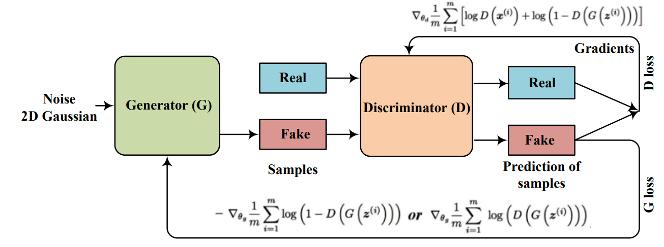
This setup is formally modeled using game theory, a field you might be familiar with from areas like economics and multi-agent systems in computer science.

The Minimax Objective Function

To implement this adversarial game, we need a single objective function that captures the competing goals of the Generator and Discriminator. This is formulated as a two-player minimax game, described by a value function, $V(G,D)$.

The Discriminator, $D$, wants to maximize this value function, which means it correctly identifies real data as real (outputting a probability close to 1) and fake data as fake (outputting a probability close to 0). The Generator, $G$, wants to minimize the same value function by producing fakes that the Discriminator mistakenly classifies as real (i.e., making $D(G(z))$ close to 1).

The following video provides an excellent and highly intuitive breakdown of this value function, connecting it directly to the binary cross-entropy loss function used in standard classification tasks.

As the video explains, the value function $V(G,D)$ is:

Let's break this down:

• ${\mathbb{E}}_{x\sim p_{\text{data}}(x)}[\log (D(x))]$: This is the expectation over real data $x$. The Discriminator wants to maximize this term, which means making $D(x)$ as close to 1 as possible for all real data.
• ${\mathbb{E}}_{z\sim p_z(z)}[\log (1-D(G(z)))]$: This is the expectation over fake data generated from noise $z$. The Discriminator also wants to maximize this term, which means making $D(G(z))$ as close to 0 as possible for all fake data.
• The Generator's objective is the opposite. It wants to minimize $V(G,D)$. Notice that $G$ only affects the second term. Minimizing this term means making $\log (1-D(G(z)))$ a large negative number, which is achieved by making $D(G(z))$ as close to 1 as possible—tricking the discriminator.

The complete optimization problem is therefore a minimax game:

The Theoretical Guarantee: Proof of Optimality

We have an objective function, but how can we be sure that reaching the equilibrium of this game achieves our ultimate goal: making the generator's distribution $p_G$ identical to the real data distribution $p_{\text{data}}$? The original GAN paper provides an elegant proof that this is indeed the case.

Given your background, walking through this proof will provide the deep theoretical grounding you're looking for. We will follow the logic presented in the "An Annotated Proof of Generative Adversarial Networks" article, which is perfectly tailored for this purpose.

The proof proceeds in two main steps:

1. For a fixed Generator $G$, we find the optimal Discriminator $D_G^{\ast }$.
2. We plug this optimal Discriminator into the objective and then find the Generator $G^{\ast }$ that minimizes this new criterion.

This proof is the theoretical bedrock of GANs. It demonstrates that the minimax game, when optimized to its global optimum, provably results in the generator learning the true data distribution.

Practical Training and Refinements

In practice, we don't solve for the optimal $D^{\ast }$ analytically. Instead, we use iterative gradient-based optimization, alternating between training the discriminator and the generator.

1. Train the Discriminator: For a fixed number of steps (often just one), we sample a minibatch of real data and a minibatch of fake data from the current generator. We then update the Discriminator's weights via gradient ascent on $V(G,D)$.
2. Train the Generator: We then freeze the Discriminator's weights and update the Generator's weights via gradient descent on $V(G,D)$.

A subtle but critical issue arises with the generator's loss function, $\mathbb{E}[\log (1-D(G(z)))]$. When the generator is poor (at the beginning of training), the discriminator easily rejects its samples, meaning $D(G(z))$ is close to 0. In this region, the gradient of $\log (1-x)$ is very small. This is the "vanishing gradient" problem: the generator gets very little feedback when it needs it most.

To overcome this, the authors proposed a modification. Instead of minimizing $\log (1-D(G(z)))$, the generator can be trained to maximize $\log (D(G(z)))$. This objective has the same fixed point but provides much stronger gradients early in training.

Conclusion

In this lesson, we have dissected the Generative Adversarial Network framework. We moved beyond the popular analogies to establish a firm theoretical understanding based on game theory and optimization.

Here are the essential takeaways:

• Adversarial Framework: GANs consist of a Generator that creates data and a Discriminator that critiques it, trained in a competitive zero-sum game.
• Minimax Objective: This game is formalized by a minimax value function $V(G,D)$, which is elegantly derived from the binary cross-entropy loss of a classifier. The discriminator seeks to maximize it, while the generator seeks to minimize it.
• Theoretical Guarantee: The core proof of GANs shows that the global minimum of this minimax game is achieved if and only if the generator's distribution $p_G$ equals the real data distribution $p_{\text{data}}$, at which point the discriminator's output is $1/2$ for all inputs.
• Practical Training: In practice, training involves alternating gradient updates. A modified, "non-saturating" loss for the generator is often used to ensure strong gradients throughout training.

You now have a solid grasp of the first principles of GANs. In our next lesson, we will turn to the final and most recent family of generative models in our survey: Diffusion Models. You will see how these models take a completely different approach, learning to generate data by systematically reversing a process of adding noise.