Diffusion Models: Iterative Denoising for Data Generation

Introduction

In our journey through generative models, we have explored two distinct philosophies. First, we examined Variational Autoencoders (VAEs), which learn an explicit probabilistic mapping from a structured latent space to the data space. Then, we delved into Generative Adversarial Networks (GANs), which reframe generation as a game-theoretic contest between a generator and a discriminator. Today, we turn our attention to the latest and arguably most powerful class of generative models: Diffusion Models.

This lesson will introduce the core principles of diffusion models. Instead of learning a direct, one-shot transformation from noise to data like GANs, or through a compact latent code like VAEs, diffusion models operate via a process of iterative refinement. You will learn about the two fundamental components of this framework: a fixed forward process that systematically corrupts data with noise, and a learned reverse process that meticulously reverses this corruption to generate new data. We will unpack the theoretical underpinnings of this method, which are rooted in thermodynamics and stochastic processes, and derive the elegant and surprisingly simple training objective that has enabled these models to achieve state-of-the-art results.

The Core Idea: Destroy and Reconstruct

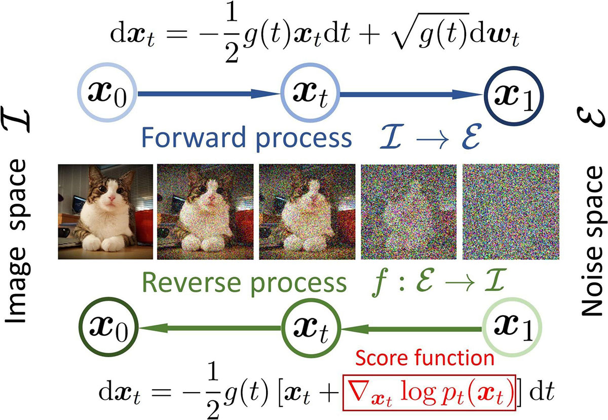
The concept behind diffusion models is both intuitive and deeply rooted in physics. Imagine taking a clear photograph and gradually adding small amounts of noise over many steps until the original image is completely indistinguishable from random static. This is the forward (diffusion) process. Now, what if we could learn to precisely reverse each of these small steps? If we could, we could start with a new image of pure random static and, by applying our learned "denoising" function repeatedly, reconstruct a clear, novel photograph. This is the reverse (denoising) process.

The following video from 3Blue1Brown's guest channel provides a superb high-level visualization of this idea, showing how pure noise is iteratively transformed into a coherent video.

This destroy-and-reconstruct paradigm is formalized using a pair of Markov chains.

The Forward Diffusion Process

The forward process, denoted by $q$, is a fixed procedure that does not involve any learning. It's defined as a Markov chain that gradually adds Gaussian noise to an image $x_0$ over $T$ discrete timesteps, according to a predefined variance schedule $\{{\beta }_t{\}}_{t=1}^T$.

At each step $t$, the new, noisier image ${\mathbf{x}}_t$ is sampled from a Gaussian distribution whose mean is a scaled version of the previous image ${\mathbf{x}}_{t-1}$ and whose variance is determined by ${\beta }_t$.

$$q({\mathbf{x}}_t|{\mathbf{x}}_{t-1})=\mathcal{N}({\mathbf{x}}_t;\sqrt{1-{\beta }_t}{\mathbf{x}}_{t-1},{\beta }_t\mathbf{I})$$

A crucial property of this process is that we can sample ${\mathbf{x}}_t$ at any arbitrary timestep $t$ directly from the original image ${\mathbf{x}}_0$, without having to iterate through all the intermediate steps. This is possible due to the properties of Gaussian distributions and is analogous to the reparameterization trick you saw with VAEs. This makes the training process highly efficient.

The following reading from Lilian Weng's highly-regarded blog post provides the mathematical derivation for this closed-form solution.

As $t$ approaches $T$, the term $\sqrt{{\bar{\alpha }}_t}$ approaches zero, meaning the final state ${\mathbf{x}}_T$ is almost entirely determined by the noise term $\mathbf{ϵ}$, effectively becoming a sample from a standard isotropic Gaussian distribution.

The Reverse Process and the Training Objective

The generative part of the model is the reverse process, $p_{\theta }$, which must learn to undo the noising steps. The goal is to learn the distribution $p_{\theta }({\mathbf{x}}_{t-1}|{\mathbf{x}}_t)$ to approximate the true but intractable reverse distribution $q({\mathbf{x}}_{t-1}|{\mathbf{x}}_t)$. We use a neural network, parameterized by $\theta$, for this task.

To train this network, we can frame the problem, much like with VAEs, as maximizing the log-likelihood of the data, which we can optimize using the variational lower bound (ELBO). The derivation is mathematically involved, but the conceptual path is what matters for your foundational understanding.

The video from the "Outlier" channel provides a clear, step-by-step walkthrough of this derivation, starting from the negative log-likelihood and arriving at the final, simplified objective function. Given your background, this detailed derivation will provide the theoretical rigor you appreciate.

As the video masterfully explains, after a long chain of theoretical derivations, we arrive at a remarkably simple and elegant training objective. Instead of predicting the denoised image ${\mathbf{x}}_{t-1}$ directly, the model ${\mathbf{ϵ}}_{\theta }$ is trained to predict the noise $\mathbf{ϵ}$ that was added to the original image ${\mathbf{x}}_0$ to create the noisy image ${\mathbf{x}}_t$.

The simplified loss function is:

$$L_{\text{simple}}={\mathbb{E}}_{t\sim [1,T],{\mathbf{x}}_0,\mathbf{ϵ}}\left[\Vert \mathbf{ϵ}-{\mathbf{ϵ}}_{\theta }({\mathbf{x}}_t,t){\Vert }^2\right]$$

Here, ${\mathbf{x}}_t$ is the noisy image created using the closed-form forward process: ${\mathbf{x}}_t=\sqrt{{\bar{\alpha }}_t}{\mathbf{x}}_0+\sqrt{1-{\bar{\alpha }}_t}\mathbf{ϵ}$. This means the training algorithm is as follows:

1. Pick a random image from your dataset, ${\mathbf{x}}_0$.
2. Pick a random timestep, $t$.
3. Generate a random noise vector, $\mathbf{ϵ}\sim \mathcal{N}(0,\mathbf{I})$.
4. Create the noisy image ${\mathbf{x}}_t$ using the formula above.
5. Feed ${\mathbf{x}}_t$ and $t$ to the neural network ${\mathbf{ϵ}}_{\theta }$.
6. Calculate the MSE between the network's output ${\mathbf{ϵ}}_{\theta }({\mathbf{x}}_t,t)$ and the original noise $\mathbf{ϵ}$.
7. Update the network's weights using gradient descent.

This objective, proposed in the Denoising Diffusion Probabilistic Models (DDPM) paper by Ho et al. (2020), was a landmark result that made diffusion models practical and powerful.

Architecture and Sampling

The final pieces of the puzzle are the model architecture and the procedure for generating new images (sampling).

Architecture

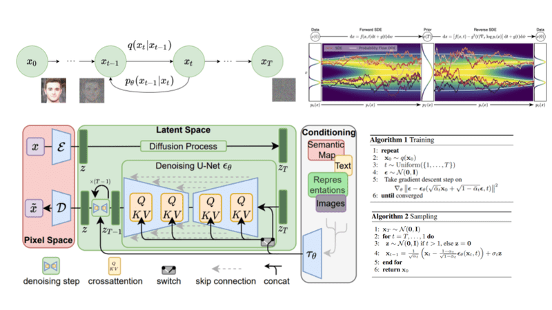
The neural network used to predict the noise, ${\mathbf{ϵ}}_{\theta }$, needs to take a noisy image and a timestep $t$ as input and output a tensor of the same shape as the input image (the predicted noise). A U-Net architecture is a natural fit for this task. U-Nets were originally developed for biomedical image segmentation and excel at image-to-image tasks. They use a series of downsampling blocks to capture context and a series of upsampling blocks with skip connections to reconstruct the image while preserving high-resolution details. The timestep $t$ is typically encoded using sinusoidal positional embeddings (the same technique from the Transformer architecture) and fed into each residual block of the U-Net.

Sampling

To generate a new image, we reverse the diffusion process:

1. Start with a tensor of pure Gaussian noise, ${\mathbf{x}}_T\sim \mathcal{N}(0,\mathbf{I})$.
2. Iterate backwards from $t=T$ down to $t=1$.
3. In each step, feed the current noisy image ${\mathbf{x}}_t$ and the timestep $t$ to the trained network ${\mathbf{ϵ}}_{\theta }$ to get a prediction of the noise.
4. Use this predicted noise to calculate the denoised image ${\mathbf{x}}_{t-1}$. An interesting detail of the original DDPM algorithm is that a small amount of stochastic noise is added back in this step, which was found to improve sample quality.
5. After $T$ steps, you are left with ${\mathbf{x}}_0$, a novel, clean image.

The Outlier video concludes with a concise summary of these two algorithms.

Conclusion

In this lesson, we have explored the fundamental principles of diffusion models, a powerful and modern approach to generative modeling. You have learned how these models elegantly combine a fixed forward process of noise injection with a learned reverse process of iterative denoising.

Here are the key theoretical takeaways:

• Core Concept: Diffusion models generate data by learning to reverse a multi-step process that gradually destroys a data sample with Gaussian noise.
• Forward Process: A fixed, non-learned Markov chain adds noise according to a predefined variance schedule. A key property is the ability to sample a noisy image at any timestep $t$ in a single, closed-form step.
• Reverse Process: A neural network (typically a U-Net) is trained to approximate the reverse (denoising) steps.
• Training Objective: Through a derivation based on the variational lower bound, the complex problem of learning the reverse distribution is simplified to an intuitive objective: training the network to predict the noise that was added at each step, using a simple Mean Squared Error loss.
• Sampling: Generation starts with pure noise and iteratively applies the trained denoising network to produce a clean sample.

This completes our survey of the three major families of generative models: VAEs, GANs, and now Diffusion Models. Each represents a unique theoretical perspective on the problem of data generation.

In the next module, we will pivot from generative modeling to a new domain of artificial intelligence: Reinforcement Learning (RL). Our first lesson will introduce the foundational concepts of RL, defining the interactive loop between an agent and its environment, and the core components of states, actions, and rewards that govern the agent's learning process.