Understanding Variational Autoencoders: ELBO and the Reparameterization Trick

Introduction

In our last lesson, we explored the standard autoencoder, establishing its function as a deterministic model for dimensionality reduction through a reconstruction objective. We saw that while excellent for data compression, its poorly structured latent space makes it unsuitable for generating new, meaningful data. Today, we advance to the Variational Autoencoder (VAE), a powerful generative model that addresses this limitation by introducing a probabilistic framework.

This lesson will guide you through the theoretical underpinnings of the VAE. You will learn how it transforms the deterministic encoder of a standard autoencoder into a probabilistic one, mapping inputs not to single points but to distributions in the latent space. We will derive its objective function, the Evidence Lower Bound (ELBO), from first principles of variational inference. Finally, we will dissect the ingenious reparameterization trick, the key that unlocks our ability to train these complex probabilistic models using standard gradient-based optimization.

From Deterministic to Generative

The core failing of a standard autoencoder as a generative model is its irregular latent space. The encoder learns to place encodings in arbitrary locations, and there's no guarantee that points sampled from the gaps between these encodings will decode into anything sensible.

VAEs solve this by imposing a structure on the latent space. Instead of learning a direct mapping $z=g(x)$, a VAE's encoder learns a mapping to a probability distribution.

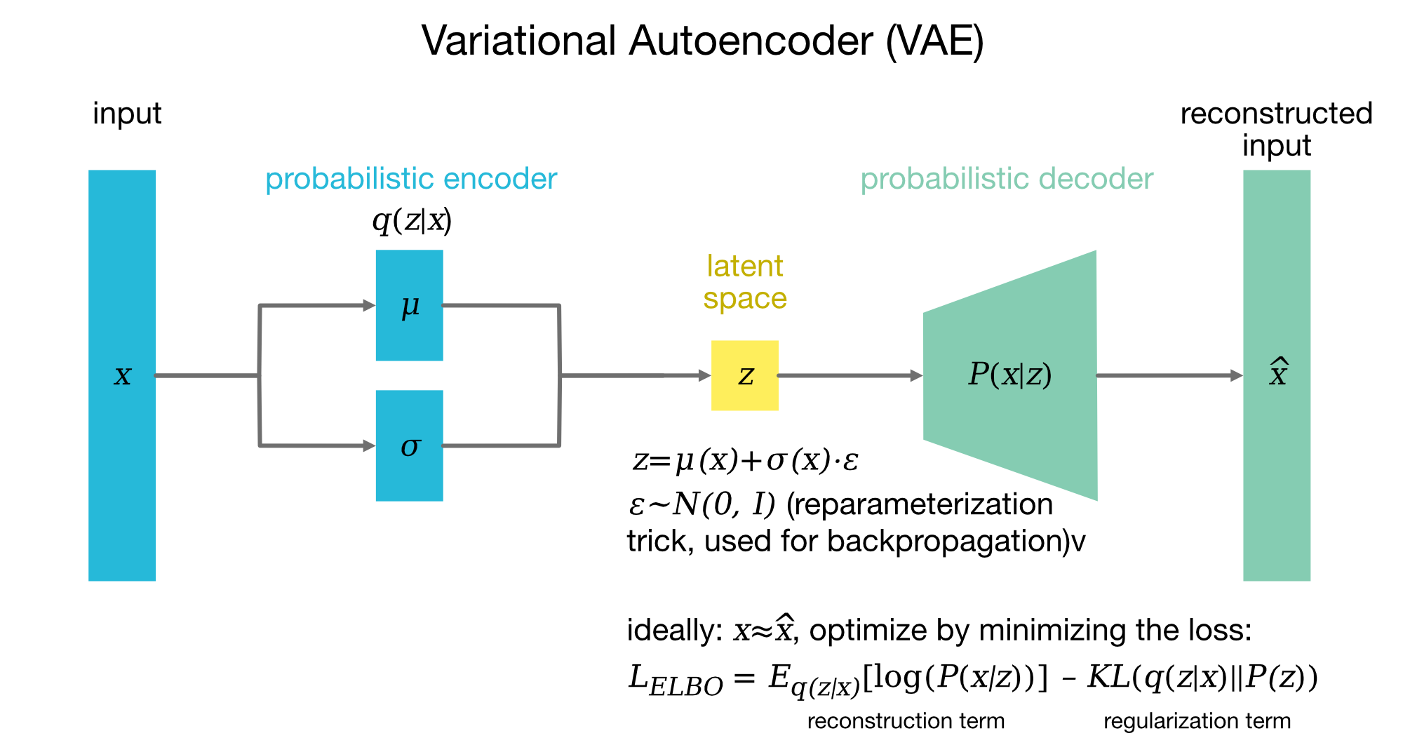
The VAE architecture reframes the encoding process:

1. Probabilistic Encoder: For an input $x$, the encoder does not produce a single latent vector $z$. Instead, it outputs the parameters of a probability distribution, typically the mean $\mu$ and the log of the variance $\log ({\sigma }^2)$ of a Gaussian distribution. This distribution, $q_{\varphi }(z|x)$, is our learned approximation of the "true" posterior.
2. Sampling: A latent vector $z$ is then sampled from this distribution: $z\sim q_{\varphi }(z|x)$.
3. Probabilistic Decoder: The decoder, $p_{\theta }(x|z)$, takes the sampled latent vector $z$ and reconstructs the original input, $\hat{x}$.

This probabilistic sampling is the essence of the VAE's generative power. It ensures that the latent space is continuous and structured, allowing us to later sample from it to generate novel data.

The Generative Goal and Variational Inference

To understand the VAE's objective function, we must first frame it in the language of probabilistic modeling. Our ultimate goal is to model the underlying distribution of our data, $p(x)$. To do this, we introduce a latent variable $z$ and model the joint distribution $p_{\theta }(x,z)=p_{\theta }(x|z)p(z)$.

• $p(z)$ is the prior distribution over the latent space. We choose this to be a simple, well-behaved distribution, typically a standard multivariate Gaussian, $\mathcal{N}(0,I)$.
• $p_{\theta }(x|z)$ is the likelihood, parameterized by a neural network (the decoder) with weights $\theta$. It defines how to generate data $x$ from a latent vector $z$.

To find the probability of our data, we would need to compute the marginal likelihood:

This integral is intractable. It requires integrating over all possible values of the high-dimensional latent space $z$, with $p_{\theta }(x|z)$ being a complex, non-linear function defined by the decoder network.

Because this is intractable, we also cannot compute the true posterior distribution $p_{\theta }(z|x)=\frac{p_{\theta }(x|z)p(z)}{p_{\theta }(x)}$, which tells us the distribution of latent variables that could have generated a given data point $x$.

This is where variational inference comes in. Since we cannot compute the true posterior $p_{\theta }(z|x)$, we approximate it with a simpler, tractable distribution $q_{\varphi }(z|x)$, which is our encoder network parameterized by $\varphi$. Our goal is to make $q_{\varphi }(z|x)$ as close as possible to the true posterior $p_{\theta }(z|x)$.

Deriving the Evidence Lower Bound (ELBO)

We measure the "closeness" between our approximation $q_{\varphi }(z|x)$ and the true posterior $p_{\theta }(z|x)$ using the Kullback-Leibler (KL) divergence. Our goal is to minimize $D_{KL}(q_{\varphi }(z|x)||p_{\theta }(z|x))$. A beautiful mathematical relationship arises when we expand this KL divergence, which leads us to our final objective function.

The following video provides an exceptionally clear, step-by-step derivation of the VAE's objective function, known as the Evidence Lower Bound (ELBO).

Let's formalize the derivation shown in the video. We start with the log-likelihood of a data point, $\log p_{\theta }(x)$, and show that it can be decomposed:

Here, $\mathcal{L}(\theta ,\varphi ;x)$ is the Evidence Lower Bound (ELBO). Because the KL divergence is always non-negative ($D_{KL}\ge 0$), we have $\log p_{\theta }(x)\ge \mathcal{L}(\theta ,\varphi ;x)$. This means that by maximizing the ELBO, we are pushing up a lower bound on the log-likelihood of our data, which is precisely our goal. Maximizing the ELBO also implicitly minimizes the KL divergence between our approximate posterior $q_{\varphi }$ and the true (but intractable) posterior $p_{\theta }(z|x)$.

The ELBO itself is further decomposed into two meaningful terms:

1. Reconstruction Term: This is the expected log-likelihood of the data, given a latent vector sampled from our encoder's distribution. It encourages the decoder to learn to reconstruct the input $x$ faithfully. For real-valued data (like images), this term often becomes a Mean Squared Error loss. For binary data, it becomes a Binary Cross-Entropy loss.

2. Regularization Term: This is the KL divergence between our approximate posterior $q_{\varphi }(z|x)$ and the prior $p(z)$. This term acts as a regularizer, forcing the distributions learned by the encoder to stay close to the simple prior (e.g., a standard normal distribution). This is the crucial component that structures the latent space, making it dense and continuous, which is exactly what we need for generation.

For a rigorous, in-depth derivation from a primary source, the original VAE paper and its subsequent tutorials are invaluable.

The Reparameterization Trick

We now have a loss function, the negative ELBO, that we want to minimize. However, there's a major technical hurdle. The reconstruction term, ${\mathbb{E}}_{z\sim q_{\varphi }(z|x)}[\log p_{\theta }(x|z)]$, involves an expectation over samples from the encoder $q_{\varphi }$. In practice, we approximate this expectation with Monte Carlo sampling (i.e., we take one sample of $z$ for each $x$).

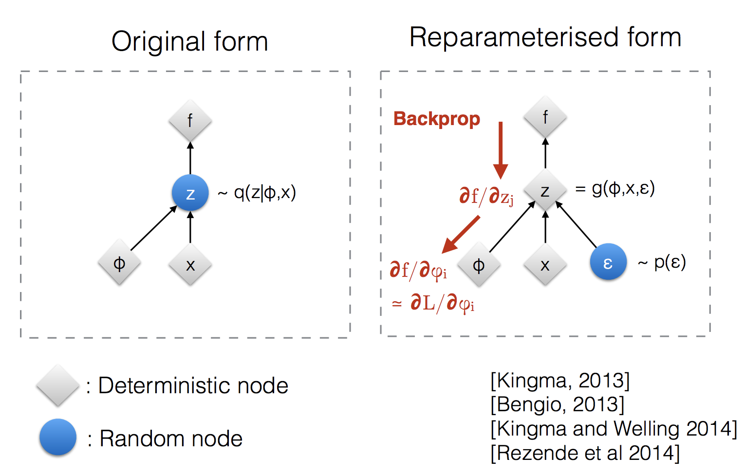
The problem is that the sampling operation, $z\sim q_{\varphi }(z|x)$, is stochastic. We cannot backpropagate gradients through a random sampling node. This would prevent us from learning the parameters $\varphi$ of the encoder. How can we differentiate with respect to $\varphi$ if the path to the loss involves a random step?

The solution is the elegant reparameterization trick. Instead of sampling directly from the distribution defined by the encoder, we externalize the randomness.

If our encoder outputs the mean ${\mu }_{\varphi }(x)$ and standard deviation ${\sigma }_{\varphi }(x)$ for a Gaussian posterior, we can reparameterize the sampling of $z$ as follows:

1. Sample a random noise vector $ϵ$ from a simple, fixed distribution: $ϵ\sim \mathcal{N}(0,I)$.
2. Compute the latent vector $z$ deterministically: $z={\mu }_{\varphi }(x)+{\sigma }_{\varphi }(x)\odot ϵ$.

The randomness now comes from $ϵ$, which is outside the computational graph of our network. The path from the encoder parameters $\varphi$ (which produce $\mu$ and $\sigma$) to the final loss is now fully deterministic and differentiable. This allows us to use standard backpropagation to train the entire VAE, including the encoder.

For the complete formal explanation, we return to the introductory paper.

Conclusion

In this lesson, we have constructed the Variational Autoencoder from its theoretical foundations. By shifting from a deterministic to a probabilistic encoder, the VAE learns not just to compress data, but to model its underlying distribution in a structured, continuous latent space suitable for generation.

Here are the key takeaways:

• Generative Goal: VAEs are generative models that aim to maximize the likelihood of the observed data, $p(x)$, by introducing a latent variable $z$.
• The ELBO: Due to the intractability of the true data likelihood, we instead maximize a lower bound called the Evidence Lower Bound (ELBO). The ELBO consists of a reconstruction term (ensuring good reconstructions) and a regularization term (structuring the latent space).
• The Reparameterization Trick: This crucial technique makes training VAEs possible. By externalizing the stochastic sampling process, it creates a differentiable path for gradients to flow through the entire network, allowing for end-to-end training with standard optimizers.

You now understand the "variational" in VAEs refers to the use of variational inference to approximate an intractable posterior, and the "autoencoder" part refers to its characteristic encoder-decoder structure.

In our next lesson, we will explore a completely different and highly influential family of generative models: Generative Adversarial Networks (GANs). You will see how GANs approach the problem of generation not through probabilistic inference and likelihoods, but through a game-theoretic, adversarial competition between two neural networks.