Autoencoder Architecture and Reconstruction for Dimensionality Reduction

Introduction

In our previous lesson, we examined how the Transformer architecture was bifurcated into encoder-only (BERT) and decoder-only (GPT) models, each specialized for language understanding and generation, respectively. Today, we shift our focus from these sequence-specific models to a more general and fundamental neural network architecture used for unsupervised learning: the autoencoder.

This lesson will explain the architecture and reconstruction objective of a standard autoencoder, a powerful tool for learning compressed representations of data, primarily for dimensionality reduction. While an "encoder" is a key component here, you will see that its purpose and interaction with a "decoder" differ significantly from the context of Transformers. We will explore how this simple yet elegant structure forces a network to learn the most salient features of data in an entirely self-supervised manner.

The Autoencoder Architecture: Learning to Reconstruct

At its core, an autoencoder is a neural network trained to perform a seemingly simple task: reconstructing its own input. It is composed of two main parts: an encoder and a decoder.

1. The Encoder: This part of the network, denoted by a function $g$, takes a high-dimensional input vector $x$ and maps it to a lower-dimensional latent representation, often called a "code" or "bottleneck," denoted by $z$. So, $z=g(x)$. The purpose of the encoder is to compress the input data into an informative, low-dimensional summary.

2. The Decoder: This part of the network, denoted by a function $f$, takes the compressed latent representation $z$ and attempts to reconstruct the original input vector. The output, denoted as $\hat{x}$, is the reconstruction: $\hat{x}=f(z)=f(g(x))$.

The entire network is trained end-to-end with the objective of making the reconstruction $\hat{x}$ as similar as possible to the original input $x$. The "bottleneck" is the crucial architectural constraint; its low dimensionality prevents the network from simply learning an identity function (i.e., copying the input to the output). Instead, it must learn to capture the most significant, essential features of the data distribution in the latent space $z$.

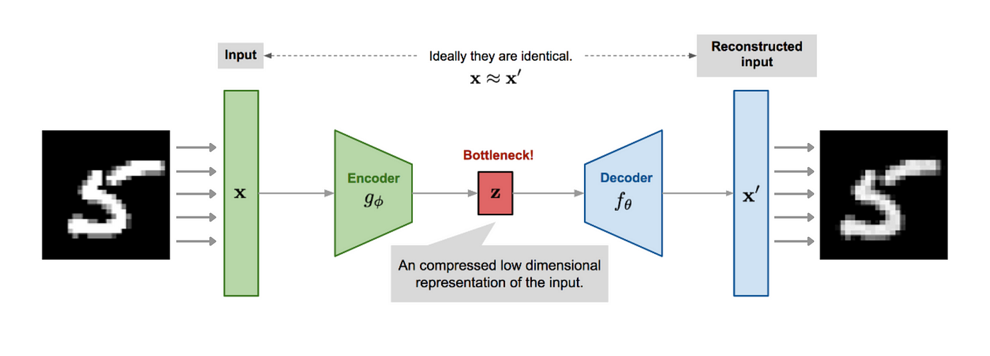
The video below offers an excellent conceptual overview of this architecture, framing it as a method for discovering an efficient "coordinate system" for complex data.

The Reconstruction Objective and Loss Functions

The training of an autoencoder is guided by the reconstruction objective, which is formalized as a loss function that measures the dissimilarity between the input $x$ and the reconstruction $\hat{x}$. The choice of loss function is critical as it is tied to the assumed statistical properties of the data. Since your background includes statistics and you have previously studied Maximum Likelihood Estimation (MLE), you will recognize that these loss functions are often derived from probabilistic principles.

Let's formalize the key points from that reading:

• Mean Squared Error (MSE): Used for continuous data (e.g., pixel intensities normalized to [0, 1]).

  $$L_{MSE}(x,\hat{x})=\frac{1}{N}\sum _{i=1}^N(x_i-{\hat{x}}_i{)}^2$$

  Minimizing MSE is equivalent to maximizing the log-likelihood of the data under the assumption that the reconstruction error, $x-\hat{x}$, follows an isotropic Gaussian distribution. This directly connects the optimization objective to the principle of MLE you studied in Module 1.

• Binary Cross-Entropy (BCE): Used for binary data ({0, 1}) or data representing probabilities ([0, 1]). For this to be well-defined, the decoder's output layer must use a sigmoid activation to ensure its outputs ${\hat{x}}_i$ are in the range (0, 1).

  $$L_{BCE}(x,\hat{x})=-\frac{1}{N}\sum _{i=1}^N[x_i\log ({\hat{x}}_i)+(1-x_i)\log (1-{\hat{x}}_i)]$$

  Minimizing BCE is equivalent to maximizing the log-likelihood assuming each input feature $x_i$ is an independent Bernoulli trial with success probability ${\hat{x}}_i$.

Case Study: Dimensionality Reduction for Document Retrieval

Once trained, the encoder provides a powerful tool for dimensionality reduction. By discarding the decoder, we can use the encoder to transform high-dimensional data points into meaningful low-dimensional vectors. These vectors can then be used for visualization, clustering, or efficient similarity search.

A classic application is document retrieval. Imagine representing millions of documents as high-dimensional "bag-of-words" vectors (e.g., 2000-dimensional vectors of word counts). Comparing a query document to all others would be computationally prohibitive. An autoencoder can be trained on these vectors to compress each document into a very low-dimensional code (e.g., 10-dimensional).

From Linear to Non-linear Dimensionality Reduction: The PCA Connection

Your study of Principal Component Analysis (PCA) in Module 6 provided a method for linear dimensionality reduction by finding the principal axes of variance in the data. There is a deep and illuminating connection between PCA and autoencoders.

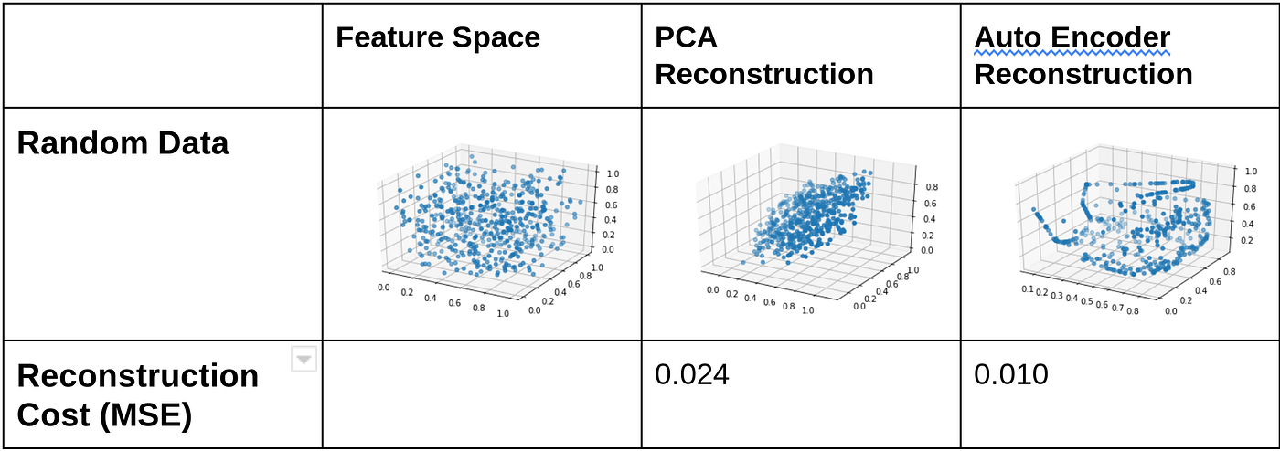
An autoencoder with a single hidden layer (the bottleneck) and linear activation functions is mathematically equivalent to PCA. Such a network learns to project the input data onto the principal subspace spanned by the top $k$ principal components, where $k$ is the dimensionality of the bottleneck.

The true power of autoencoders is unlocked when we introduce non-linear activation functions (e.g., ReLU, sigmoid, tanh) into the encoder and decoder layers. By doing so, the autoencoder is no longer restricted to learning a linear subspace. Instead, it can learn to project data onto a low-dimensional, curved non-linear manifold. This makes autoencoders a powerful generalization of PCA.

The following videos provide a formal explanation of this connection and its implications.

The difference between linear and non-linear dimensionality reduction is profound. While PCA might find the best flat plane to approximate a coiled "Swiss roll" dataset, a non-linear autoencoder can learn to "unroll" it onto a simple 2D plane, preserving the intrinsic structure of the data much more effectively.

Conclusion

In this lesson, we have established the theoretical foundation of the standard autoencoder. You now understand its architecture, its training objective, and its primary function as a tool for unsupervised dimensionality reduction.

Key takeaways from our discussion include:

• Architecture: An autoencoder consists of an encoder that maps data to a low-dimensional bottleneck (latent space), and a decoder that reconstructs the original data from this compressed representation.
• Reconstruction Objective: The network is trained by minimizing a reconstruction loss that measures the difference between the input $x$ and the output $\hat{x}$. Common choices are MSE (for continuous data, assuming Gaussian error) and BCE (for binary data, assuming Bernoulli distributions).
• Dimensionality Reduction: Autoencoders learn to compress data in a way that preserves its most salient features, making them a powerful non-linear generalization of PCA. While a linear autoencoder learns a principal subspace, a non-linear autoencoder learns a principal manifold.

The standard autoencoder is a deterministic model: for a given input $x$, the encoder will always produce the exact same latent code $z$. This is excellent for compression, but less useful for generation. What if we wanted to sample new points from the latent space to generate novel data? This requires a probabilistic approach.

In our next lesson, we will build directly upon this foundation to explore the Variational Autoencoder (VAE). You will learn how VAEs introduce a probabilistic framework to the latent space, transforming the autoencoder from a simple compression tool into a powerful generative model.