Learning Rate Scheduling Techniques

Hello! Let's dive into our next lesson on improving deep learning model training.

Introduction

In our previous lessons, we assembled the core components of a training pipeline. We learned about optimizers like SGD and Adam, which define how to update model weights, and we explored weight initialization strategies like Xavier and He, which determine where the optimization process begins.

Today, we address another critical hyperparameter: the learning rate. You've seen it as a fixed value passed to the optimizer, but keeping it constant throughout training is often not the best approach. In this lesson, we will explore learning rate scheduling, a powerful technique for dynamically adjusting the learning rate to improve training speed and model performance.

Our learning outcome is to apply learning rate scheduling strategies during training. We'll cover why this is important and then explore several common strategies, from simple decay schedules to more adaptive methods, and see how to implement them in PyTorch.

1. The Problem with a Fixed Learning Rate

The learning rate controls the size of the steps your optimizer takes in the loss landscape. Choosing the right value is a delicate balance:

• A learning rate that's too high can cause the optimizer to overshoot the minimum, leading to unstable training where the loss bounces around or even diverges.
• A learning rate that's too low makes training painfully slow and increases the risk of getting stuck in a suboptimal local minimum.

Even with a well-chosen fixed learning rate, the optimal step size changes during training. In the beginning, when the model is far from a solution, larger steps are beneficial for faster progress. However, as training progresses and the model approaches a good solution in the loss landscape, we need to take smaller, more careful steps to "settle" into the minimum without overshooting it.

This video provides an excellent visual recap of this trade-off and introduces the idea of scheduling.

As the video explains, the solution is to start with a relatively high learning rate and decrease it over time. This process is called learning rate annealing or decay, and the strategy we use to manage it is a learning rate scheduler.

2. Common Learning Rate Scheduling Strategies

PyTorch provides a convenient torch.optim.lr_scheduler module with implementations of many common scheduling policies. Let's explore some of the most widely used ones.

A scheduler is typically tied to an optimizer. You create it after your optimizer and then call its step() method at the end of each epoch (or sometimes, each batch) to update the learning rate.

# General pattern
optimizer = torch.optim.Adam(model.parameters(), lr=0.01)
scheduler = torch.optim.lr_scheduler.SomeScheduler(optimizer, ...) # Initialize the scheduler

for epoch in range(num_epochs):



    # Training loop...
    for batch in train_loader:



        # ... forward pass, loss, backward pass
        optimizer.step()




    # After the epoch (or sometimes after validation)
    scheduler.step()

Now, let's examine specific schedulers.

Step-Based Decay

These schedulers decrease the learning rate based on a pre-defined schedule tied to the number of epochs.

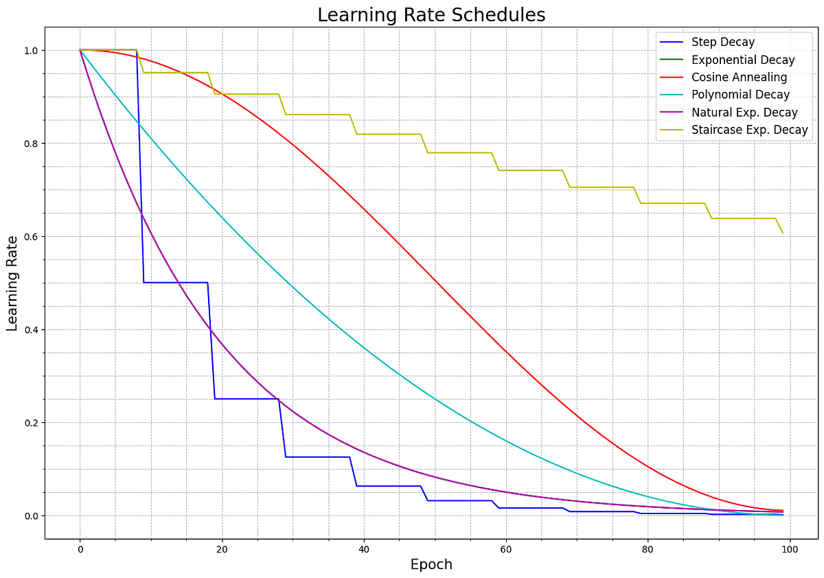
• StepLR: This is one of the simplest schedulers. It decays the learning rate by a multiplicative factor (gamma) every step_size epochs. For example, you could halve the learning rate every 10 epochs.
• MultiStepLR: A more flexible version of StepLR. It decays the learning rate by gamma at specific, manually defined epoch numbers (milestones). This is useful if you observe that your model's improvement tends to plateau at certain points.
• ExponentialLR: This scheduler decays the learning rate by gamma after every epoch.

The following resource gives a great visual overview of these schedulers and many others.

Performance-Based Decay: ReduceLROnPlateau

Instead of following a fixed schedule, it's often more effective to adapt the learning rate based on the model's performance. ReduceLROnPlateau is a very popular and intuitive scheduler that does exactly this.

It monitors a metric, typically the validation loss. If this metric stops improving for a certain number of epochs (defined by patience), the scheduler reduces the learning rate by a multiplicative factor. This approach "waits" for training to stagnate before making an adjustment.

Unlike other schedulers, its step() method is called with the metric you're monitoring: scheduler.step(validation_loss).

Curve-Based Schedulers: CosineAnnealingLR

This has become a very popular and effective default choice. Instead of sharp drops, CosineAnnealingLR smoothly anneals the learning rate from its initial value down to a minimum value (eta_min) following the shape of a cosine curve. This avoids the abrupt changes of step-based schedulers and allows for a gradual fine-tuning process as training progresses.

To see how these different strategies are implemented in PyTorch and how they fit into the training loop, let's watch a practical tutorial.

3. A Note on Warmup

A final useful technique to be aware of is warmup. In the very early stages of training, when the model's weights are still random, large learning rates can lead to instability. A warmup period addresses this by starting with a very small learning rate and gradually increasing it to the initial target learning rate over a few epochs. After the warmup phase, the main learning rate schedule (e.g., cosine annealing or step decay) takes over.

This helps prevent the optimizer from taking excessively large and misguided steps at the beginning, leading to more stable training, especially in very deep or complex models like Transformers.

The "Dive into Deep Learning" book provides a clear explanation and visualization of this concept.

Conclusion

You've now learned how to go beyond a fixed learning rate to implement dynamic adjustments that can significantly improve your model's training.

Key Takeaways:

• Fixed learning rates are suboptimal: The ideal learning rate changes as training progresses.
• Learning rate schedulers automate the process of adjusting the learning rate. This generally leads to faster convergence and a lower final loss.
• Common strategies include:
  • Step-based decay (StepLR, MultiStepLR): Simple and effective. Reduces LR at fixed intervals.
  • Performance-based decay (ReduceLROnPlateau): An adaptive strategy that reduces LR when validation performance stagnates.
  • Cosine Annealing (CosineAnnealingLR): A popular and robust method that smoothly decays the LR along a cosine curve.
• Warmup is a useful complementary technique that stabilizes training in the initial epochs by starting with a small LR and gradually increasing it.
• In PyTorch, you attach a scheduler to an optimizer and call scheduler.step() within your training loop (usually at the end of each epoch).

In our next lesson, we'll focus on how to monitor and diagnose the training process. We will learn how to identify overfitting by analyzing training and validation loss curves, which is precisely how you would observe the benefits of a well-chosen optimizer and learning rate schedule.