Understanding Weight Initialization: Xavier and He Methods

Hello! Welcome to your next lesson on training deep neural networks.

Introduction

In our last lesson, we explored the role of optimizers like Adam and SGD, which are the engines that drive learning by updating model weights to minimize loss. We saw that the training process is an iterative search for the best set of weights. This raises a fundamental question: where does this search begin?

This lesson focuses on weight initialization, the process of setting the initial values for the weights in a neural network. It might seem like a minor detail, but as you'll see, the choice of initial weights is critical. A poor choice can prevent a deep network from learning at all, while a good choice can significantly speed up convergence and improve performance.

Our goal is to explain the purpose of weight initialization strategies, focusing on two modern standards: Xavier and He initialization. We will first explore what happens when initialization goes wrong, and then see how these principled methods provide a solution.

1. The Perils of Poor Initialization

Before we learn the right way to initialize weights, it's crucial to understand why simple approaches fail. Let's examine a few common but flawed strategies.

The Symmetry Problem: Zero or Constant Initialization

What if we initialize all weights to zero? Or to a constant value like 0.5? This seems simple, but it creates a fatal issue known as the symmetry problem.

If all weights are the same, every neuron in a given layer will receive the same inputs, perform the same computation, and produce the same output. During backpropagation, they will also receive the same gradient and thus undergo the exact same update. This symmetry is never broken.

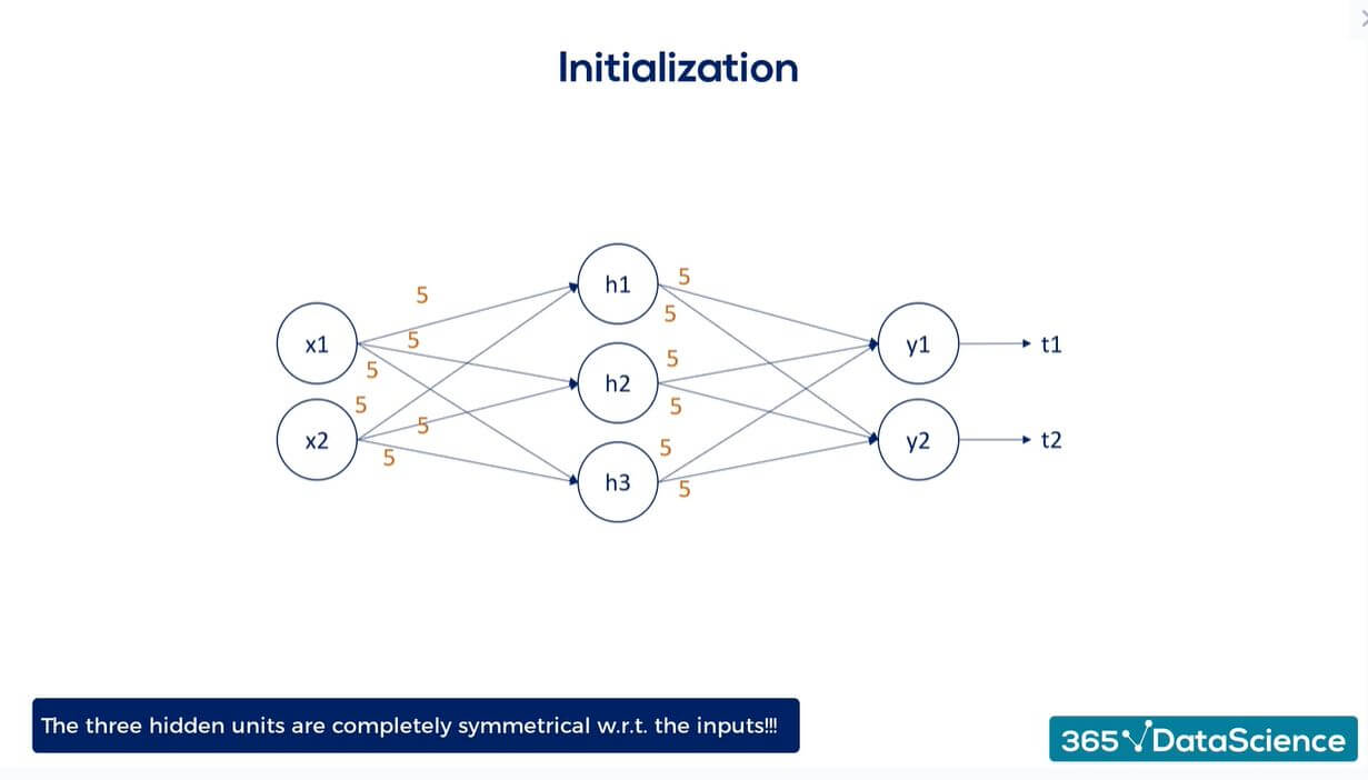
This means that no matter how many neurons you have in a layer, they all learn the same thing. The network's ability to learn complex, hierarchical features is completely crippled.

The Gradient Problem: Small or Large Random Values

A natural next step is to break the symmetry by using small random numbers. While this solves the symmetry problem, it introduces new issues in deep networks:

• Vanishing Gradients: If weights are too small, the weighted sum of inputs will be small. For activation functions like tanh or sigmoid, this keeps the activations near zero. As this small signal propagates through many layers, it diminishes further, causing the gradients during backpropagation to become vanishingly small. The early layers of the network learn extremely slowly, if at all.
• Exploding Gradients: If weights are too large, the opposite happens. The activations can grow exponentially with each layer, leading to enormous values. This causes the gradients to become huge, making the weight updates unstable and causing the training process to diverge.
• Saturation: With large weights, the inputs to sigmoid or tanh functions can be far from zero, pushing the output to the "saturated" flat parts of the curve (near -1/1 for tanh, or 0/1 for sigmoid). In these regions, the gradient is almost zero, which again stalls learning.

To understand these failure modes in more detail, let's read an article that explains them clearly.

2. The Solution: Controlling Signal Variance

The core insight behind modern initialization techniques is that we need to keep the variance of the activations and gradients consistent as they propagate through the network. We want to avoid the signal either dying out (vanishing) or blowing up (exploding).

The key is to scale the initial weights based on the number of input and output neurons for a layer. We define:

• fan_in: The number of input connections to a neuron (i.e., the number of neurons in the previous layer).
• fan_out: The number of output connections from a neuron (i.e., the number of neurons in the current layer).

The intuition is simple: if a neuron has a large number of inputs (fan_in), the random weights connected to it should be smaller to keep the variance of its output under control. This insight is the foundation for both Xavier and He initialization.

3. Xavier (Glorot) Initialization

Xavier initialization, named after Xavier Glorot, was designed to work well with saturating activation functions like tanh and sigmoid. It balances the fan_in and fan_out to ensure the variance of the activations and backpropagated gradients remains roughly constant from layer to layer.

The strategy is to draw weights from a distribution with a mean of 0 and a specific variance.

To get a quick and clear overview of this method, let's watch a short video.

As you saw, the goal is to set the variance of the weights $\text{Var}(W)$ based on the layer's size. The two common forms of Xavier initialization are:

1. Xavier Normal: Draw weights from a normal distribution with mean 0 and variance ${\sigma }^2=\frac{2}{fa{n}_{in}+fa{n}_{out}}$.
2. Xavier Uniform: Draw weights from a uniform distribution $U[-b,b]$, where $b=\sqrt{\frac{6}{fa{n}_{in}+fa{n}_{out}}}$.

This method was a significant step forward, but its derivation relies on assumptions (like linear activations) that don't hold true for the most common activation function used today: ReLU.

4. He Initialization

When using the Rectified Linear Unit (ReLU) activation function, a different approach is needed. Since ReLU sets all negative inputs to zero, it effectively "kills" about half of the activations. This changes the variance of the outputs in a way that Xavier initialization doesn't account for, which can lead to vanishing gradients again.

He initialization, named after Kaiming He, was developed specifically for ReLU and its variants (like Leaky ReLU). It compensates for the zeroing effect of ReLU by using a larger variance for the weights.

Let's see how this method is derived and why it's better for ReLU.

The formulas for He initialization are similar to Xavier's but only consider fan_in:

1. He Normal: Draw weights from a normal distribution with mean 0 and variance ${\sigma }^2=\frac{2}{fa{n}_{in}}$.
2. He Uniform: Draw weights from a uniform distribution $U[-b,b]$, where $b=\sqrt{\frac{6}{fa{n}_{in}}}$.

Notice the variance is roughly double that of Xavier initialization, which helps keep the signal strong enough when passing through ReLU layers.

For a final recap and to see the formulas laid out clearly, this article is an excellent reference.

Conclusion

In this lesson, we uncovered why careful weight initialization is not just a minor tweak but a fundamental requirement for training deep neural networks.

Key Takeaways:

• Bad initialization is fatal: Initializing weights to zero or a constant causes a symmetry problem, crippling the network. Initializing them randomly but improperly (too small or too large) leads to vanishing or exploding gradients.
• The solution is variance control: The goal of modern initialization is to set the initial weights such that the variance of the signal (activations and gradients) remains stable as it propagates through the network.
• Xavier (Glorot) Initialization is designed for saturating activation functions like tanh and sigmoid. It scales weights based on both the number of input (fan_in) and output (fan_out) neurons.
• He Initialization is the standard for ReLU and its variants. It accounts for ReLU's non-linearity by using a larger variance, typically based only on fan_in.

As a simple rule of thumb: if you are using ReLU activations, start with He initialization. If you are using tanh or sigmoid, use Xavier. Most modern deep learning frameworks make these the default choices for their respective layers.

In our next lesson, we will continue exploring techniques to improve training by looking at learning rate scheduling, a method to dynamically adjust the learning rate during training to achieve faster convergence and better final performance.