Simple Resistive Circuits: KCL, KVL, and Ohm's Law

Hello! Welcome to your next lesson on circuit analysis.

In the last lesson, we developed a powerful qualitative understanding of how circuits behave. We saw that changes propagate through a circuit via transient waves of surface charge, which ultimately settle into a new stable state. We learned to predict the direction of these changes using limiting cases and VIRP tables.

Today, we will bridge the gap from qualitative prediction to quantitative analysis. Your goal for this lesson is to solve a simple resistive circuit by combining physical reasoning with KCL, KVL, and Ohm's law. We will translate the physical laws we've explored into a system of equations to find the exact voltages and currents in a circuit. Your intuitive predictions will now serve as an essential tool for verifying that your calculated results make physical sense.

1. From Physical Laws to a Problem-Solving Framework

Solving a circuit is a logical process, much like debugging a program or solving a puzzle. We start with fundamental truths (KCL, KVL, Ohm's law) and apply them systematically to find the unknown variables.

Here is a reliable, step-by-step framework for analyzing any resistive circuit:

1. Label the Circuit:

   • Nodes: Identify and label all the points where components connect. It's helpful to choose one node as the "ground" or reference (0V). This simplifies voltage calculations.
   • Currents: Assign a current variable (e.g., $I_1,I_2$) and an assumed direction to each branch of the circuit. A branch is a path between two nodes containing one or more components in series.
   • Voltages: Mark the polarity (+ and -) of the voltage drop across each resistor. By convention, current flows from the positive to the negative terminal of a resistor.

2. Formulate Equations:

   • KCL: Apply Kirchhoff's Current Law ($\sum I_{in}=\sum I_{out}$) at n-1 of the n nodes in your circuit. This ensures charge is conserved.
   • KVL: Apply Kirchhoff's Voltage Law (the algebraic sum of voltage changes around a closed loop is zero) for enough independent loops to have a complete set of equations. The number of independent loops is equal to the number of branches minus the number of nodes plus one.

3. Solve the System:

   • You will now have a system of linear equations where the number of equations equals the number of unknown currents.
   • Solve this system using algebraic methods like substitution or elimination.

The most crucial and error-prone step is applying KVL correctly. Let's solidify the sign conventions.

2. Mastering the Signs for KVL

When you "walk" around a circuit loop to apply KVL, you are summing up the voltage changes. Think of it like walking up and down hills on a hike.

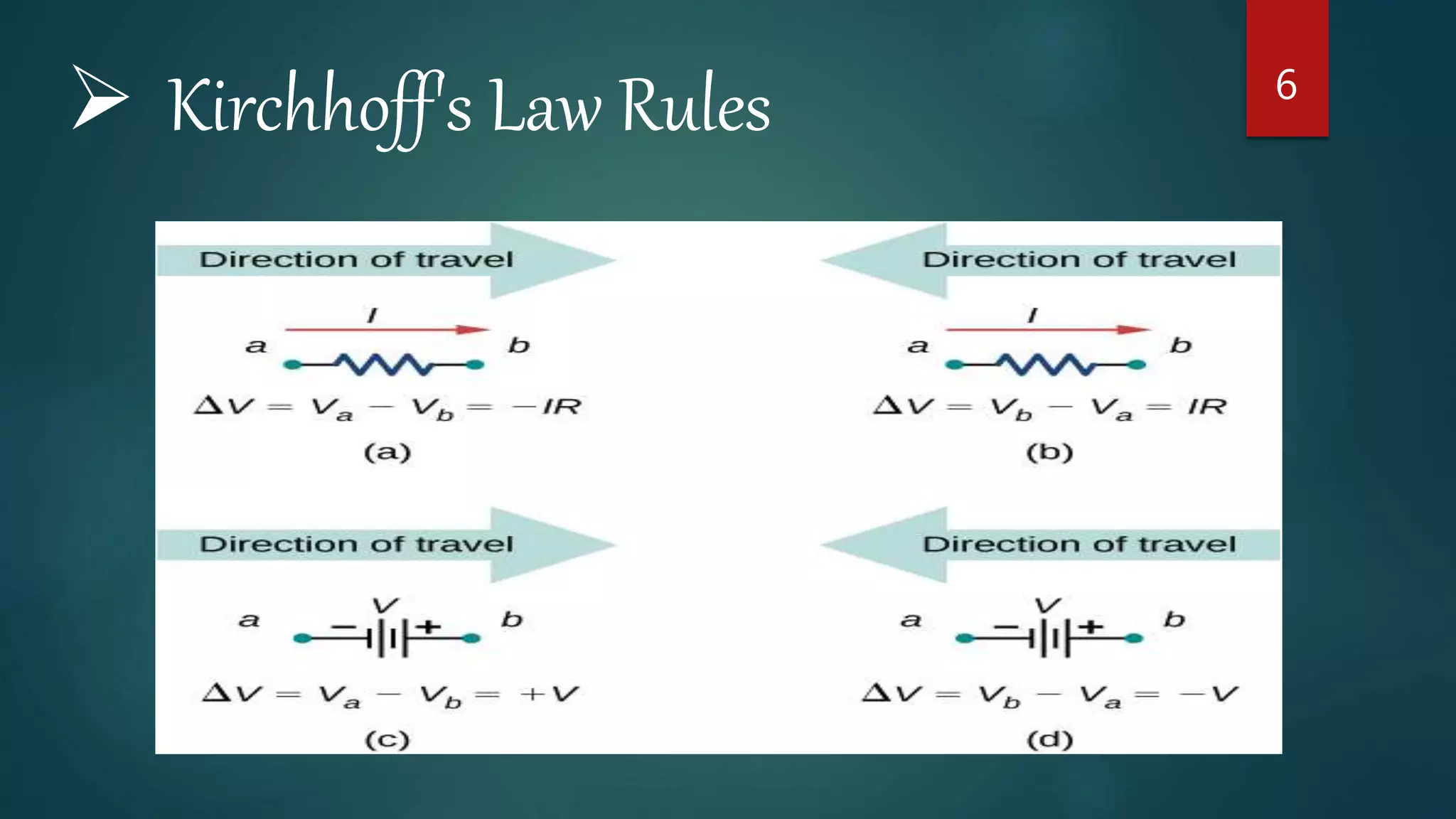
Here's how to apply this:

• For a Resistor:

  • If you travel with the assumed current direction, you are moving from high potential to low potential. This is a voltage drop, so the change is negative ($-IR$).
  • If you travel against the assumed current direction, you are moving from low potential to high potential. This is a voltage rise, so the change is positive ($+IR$).

• For a Voltage Source:

  • If you travel from the negative to the positive terminal, you are gaining potential. This is a voltage rise, so the change is positive ($+V$).
  • If you travel from the positive to the negative terminal, you are losing potential. This is a voltage drop, so the change is negative ($-V$).

By consistently applying these rules, you can confidently build the correct KVL equations.

3. A First Example: The Series Circuit

Let's apply this framework to a simple series circuit. Our goal is to find the current flowing through the circuit and the voltage drop across each resistor.

1. Label the Circuit:

• Nodes: There are technically three nodes, but since it's one continuous loop, there's only one path for current.
• Current: There is only one current, $I$. Let's assume it flows clockwise, out of the positive terminal of the source.
• Voltages: The voltage drops across the resistors will be $V_1$, $V_2$, and $V_3$, with the positive side where the current enters.

2. Formulate Equations:

• KCL: With only one path, KCL is trivial; the current is the same everywhere.
• KVL: Let's start at the bottom-left corner and walk clockwise around the loop.
  • Through the 20V source: We go from - to +. This is a rise: $+20V$.
  • Through R1 (15Ω): We go with the current. This is a drop: $-I\cdot 15\Omega$.
  • Through R2 (20Ω): We go with the current. This is a drop: $-I\cdot 20\Omega$.
  • Through R3 (5Ω): We go with the current. This is a drop: $-I\cdot 5\Omega$.
  • The sum must be zero: $$20-15I-20I-5I=0$$

3. Solve the System:

• Combine the terms: $$20-(15+20+5)I=0$$ $$20-40I=0$$
• Solve for $I$: $$I=\frac{20V}{40\Omega }=0.5A$$ Since the result is positive, our assumed clockwise direction was correct.

Now, we can find the voltage drop across each resistor using Ohm's Law ($V=IR$):

• $V_1=0.5A\cdot 15\Omega =7.5V$
• $V_2=0.5A\cdot 20\Omega =10.0V$
• $V_3=0.5A\cdot 5\Omega =2.5V$

Notice that $7.5V+10.0V+2.5V=20V$. The total voltage dropped by the resistors exactly equals the voltage supplied by the source, satisfying KVL and confirming our energy conservation intuition.

4. A Multi-Loop Circuit Analysis

Now for a more interesting puzzle: a circuit that can't be simplified by combining series/parallel resistors. This is where the full power of KCL and KVL becomes apparent.

After watching the video, let's reflect on the process.

• Arbitrary Directions: The initial choice of current directions is arbitrary. If you solve for a current and get a negative value (e.g., -2A), it doesn't mean you made a mistake. It simply means the actual current of 2A flows in the direction opposite to the one you initially drew on your diagram.
• Independence: We needed three unknowns ($I_1,I_2,I_3$), so we needed three independent equations. Using KCL at node B gave us one. Using KVL on the two inner loops gave us the other two. Using KCL at node D or KVL on the outer loop would have given us a redundant equation—one that is just a combination of the others—so it wouldn't have helped solve the system.

This process transforms a complex circuit problem into a solvable system of linear equations—a problem your algebra skills are well-equipped to handle.

Conclusion

In this lesson, you've learned to translate your intuitive understanding of circuit physics into a rigorous, quantitative problem-solving method. By systematically labeling a circuit, applying the fundamental conservation laws of KCL and KVL, and using Ohm's Law, you can determine the precise voltage and current for every component.

Key Takeaways:

• Framework is Key: A structured approach (Label, Formulate, Solve) removes ambiguity and minimizes errors.
• Sign Conventions are Crucial: Consistently applying the sign conventions for voltage rises and drops is essential for building correct KVL equations.
• Math as a Tool for Physics: The algebra used to solve the system of equations is simply a tool to find the specific values that satisfy the underlying physical laws of energy and charge conservation.
• Negative Answers are Informative: A negative result for a current indicates its actual direction is opposite to your initial assumption.

Preview of the Next Lesson:
We have focused on combining resistors in series and parallel conceptually and have now used a full KCL/KVL analysis. In the next lesson, we will formalize the process of circuit simplification. We'll derive the formulas for equivalent resistance of series and parallel combinations and see how they arise directly from KCL and KVL. This will give you a powerful shortcut for simplifying many circuits before applying a full analysis.