Circuit Changes: Current & Voltage Redistribution

Recommended resources

The freely available resources this lesson will direct you to.

Hello! Welcome to the third lesson in our module on circuit conservation laws.

In our previous lessons, we established the two fundamental rules governing circuit behavior:

Kirchhoff's Current Law (KCL): Based on the conservation of charge, it tells us that current is conserved at any junction (node).
Kirchhoff's Voltage Law (KVL): Based on the conservation of energy, it tells us that the sum of voltage changes around any closed loop must be zero.

These laws are perfect for analyzing a circuit in a stable, or "steady," state. But this raises a fascinating question, one that gets to the very heart of circuit intuition: If you change one component in a circuit, how do all the other parts "know" to adjust? How does the information about the change propagate and cause the entire system to settle into a new steady state that still obeys KCL and KVL?

Your goal for this lesson is to learn how to qualitatively predict how current and voltage redistribute when a component is added to or removed from a simple circuit. We'll go beyond the static rules and explore the dynamic physical process that underlies these changes, building the deep, logical mental model you're looking for.

1. The Unseen Process: Transients and Surface Charges

Textbooks often present circuit laws as if they are instantaneously true everywhere. But this would require information to travel infinitely fast, which we know is impossible. The real answer lies in a very brief, chaotic period called the transient phase, which is usually over in nanoseconds. Understanding this phase is the key to unlocking true circuit intuition.

Why resistors in series have different voltage (but same current)?

The video 'Why resistors in series have different voltage (but same current)?' from the FloatHeadPhysics channel provides a brilliant explanation of this hidden process. It dives into the moments just after a switch is closed to reveal the mechanism that circuits use to self-organize.

Watch the entire video (up to 14:34). It's dense with conceptual insights, so pay close attention to this sequence of events: Initial Chaos (01:28): In the first instant, the current is not the same everywhere. It's high in the low-resistance wires and low in the resistors. Charge Accumulation (03:10): This uneven flow causes a 'traffic jam' of electrons, leading to a buildup of negative charge on one side of a resistor and a deficit (positive charge) on the other. These are called surface charges. Field Redistribution (06:20): These new pockets of charge create their own electric fields, which superimpose on the original field from the battery. This new, combined field is what alters the forces on all the electrons in the circuit. Reaching Equilibrium (08:46): The process continues—currents adjusting, charges re-accumulating—until the forces balance in such a way that the current becomes uniform throughout the loop. The accumulated surface charges are what create the final, steady-state voltage drops across the resistors.

This is the physical mechanism you were looking for. A change in any part of the circuit (like adding a resistor) alters the flow pattern, which causes surface charges to redistribute. This redistribution changes the electric field everywhere in the circuit, which in turn guides the currents into a new, stable equilibrium. It's a beautiful, self-correcting system.

This concept of a gradient in surface charge density being the direct cause of the electric field that drives the current is a powerful mental model. A steeper gradient (a rapid change in charge density over a short distance) creates a stronger field and a larger voltage drop, which is exactly what happens across a high-value resistor.

2. Visualizing Redistribution: Potential as a Landscape

Now that we have the microscopic picture of surface charges, let's use a macroscopic analogy to visualize how potential (voltage) redistributes across the "landscape" of a circuit.

An intuitive approach for understanding electricity

The video 'An intuitive approach for understanding electricity' by AlphaPhoenix uses a fantastic water trough analogy to make the concept of electric potential tangible.

First, watch from the beginning to 01:49. Notice how adding a single resistor transforms a smooth, gradual drop in potential into a sudden, sharp 'step'. \nNext, watch the segment from 19:49 to 24:21. Here, the water level represents electric potential. Observe how placing an obstacle (a resistor) in the trough forces the water level (potential) to 'pile up' behind it, creating a step change, while remaining relatively flat elsewhere.

This analogy helps visualize the end state. But what about the dynamic process of getting there? When we change a component, the potential landscape doesn't just instantly reconfigure itself. It "sloshes" around and settles, just like the surface charges we saw earlier.

Let's see this dynamic redistribution in action.

An intuitive approach for understanding electricity

The same video from AlphaPhoenix has a wonderful segment that demonstrates this dynamic process. He pulls a blocker out of the water stream, simulating the closing of a switch or the removal of a high resistance.

Watch from 30:01 to 31:15. Observe how the removal of the blocker sends a wave through the system, which reflects and sloshes around before settling into a new, stable water level distribution. This is a physical analog of the electrical transient phase, where the circuit finds its new equilibrium.

3. A Systematic Method for Qualitative Prediction

Building physical intuition is the goal, but we also need a structured way to apply it. The document from the "Modular Electronics Learning (ModEL) project" provides excellent techniques for this kind of qualitative reasoning.

One of the most powerful strategies is to use limiting cases. To predict what happens when a resistor's value increases, you can analyze the extreme case of it increasing to infinity (an open circuit). To predict what happens when it decreases, you can analyze the extreme case of it dropping to zero (a short circuit). The direction of change will be the same.

[PDF] "Modular Electronics Learning (ModEL) project" - Ibiblio

Let's explore this idea of limiting cases and other formal methods for qualitative analysis. This document explains the principles and provides a structured format for your reasoning.

This is a detailed document, so we'll focus on a few key sections: Read Section 3.4, 'Review of opens and shorts' (Page 24). Pay close attention to the definition of an open (zero current) and a short (zero voltage) and how they can be used as limiting cases for analysis. Skim Section 2.1, 'Example: potential in open and shorted circuits' (Pages 8-14). Look at the color-coded diagrams. See how introducing an open or a short drastically redistributes the potential (the colors) in the circuit. This reinforces the AlphaPhoenix video's visualization. Study Section 2.2, 'Example: qualitative VIRP table usage' (Pages 15-16). This introduces a fantastic tool for structured reasoning. The VIRP (Voltage, Current, Resistance, Power) table lets you trace the consequences of a single change throughout a circuit using only arrows (↑, ↓, or 'same'). This method transforms qualitative prediction into a logical puzzle.

Let's walk through the logic of the VIRP table from the reading.

Given: In a parallel circuit, $R_{2}$ decreases (↓). Source voltage and other resistors are constant.
Step 1 (Properties of Parallel Circuits): Since all components are in parallel, their voltage must be the same as the source. So $V_{1}$ , $V_{2}$ , and $V_{3}$ are all constant.
Step 2 (Ohm's Law, $I = V / R$ ):
- For $R_{1}$ and $R_{3}$ : $V$ is constant, $R$ is constant $⟹$ $I_{1}$ and $I_{3}$ are constant.
- For $R_{2}$ : $V_{2}$ is constant, $R_{2}$ decreases $⟹$ $I_{2}$ must increase (↑).
Step 3 (KCL at a Node): Total current $I_{t o t a l} = I_{1} + I_{2} + I_{3}$ . Since $I_{1}$ and $I_{3}$ are constant and $I_{2}$ increases, $I_{t o t a l}$ must increase (↑).

This step-by-step causal chain is exactly the kind of rigorous, logical thinking that builds robust intuition.

4. Practice Your Predictive Power

Let's apply these ideas to a circuit. Consider the following diagram. The switch S is initially closed.

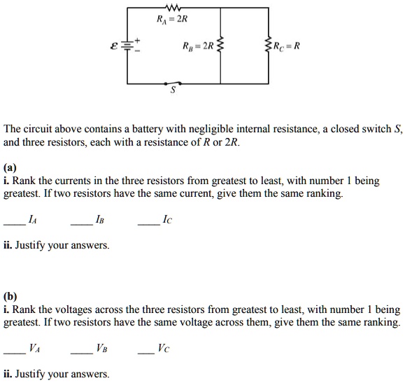
Resistive Circuit Analysis Problem: Ranking Currents and Voltages — Circuit with resistors R_A = 2R, R_B = 2R, and R_C = R. R_A is in series with the parallel combination of R_B and R_C.

Thought Experiment: Imagine the switch S is closed, and the circuit is in a steady state. Now, what happens to the voltage across $R_{A}$ ( $V_{A}$ ) and the current through $R_{C}$ ( $I_{C}$ ) if resistor $R_{B}$ is suddenly removed (i.e., its branch "fails open")?

Try to reason through this step-by-step, using the principles we've discussed. You can even set up a qualitative VIRP table.

Click to see the step-by-step reasoning.

Initial State: Current from the source flows through $R_{A}$ , then splits between $R_{B}$ and $R_{C}$ .
The Change: The path through $R_{B}$ is opened. This is the limiting case of $R_{B}$ 's resistance going to infinity.
Effect on Resistance:
- The parallel combination of $R_{B}$ and $R_{C}$ is replaced by just $R_{C}$ .
- The equivalent resistance of the parallel part was $R_{p a r a l l e l} = (R_{B} \cdot R_{C}) / (R_{B} + R_{C}) = (2 R \cdot R) / (2 R + R) = \frac{2}{3} R$ .
- The new resistance of that part of the circuit is just $R_{C} = R$ .
- Since $R > \frac{2}{3} R$ , the resistance of this section has increased.
- The total circuit resistance is $R_{t o t a l} = R_{A} + R_{e q u i v a l e n t}$ . Since $R_{A}$ is constant and $R_{e q u i v a l e n t}$ increased, the total resistance of the circuit increases.
Effect on Total Current ( $I_{t o t a l}$ ):
- From Ohm's Law, $I_{t o t a l} = V_{so u r ce} / R_{t o t a l}$ .
- Since $V_{so u r ce}$ is constant and $R_{t o t a l}$ increased, the total current decreases.
Effect on $V_{A}$ :
- The current through $R_{A}$ is the total current, $I_{A} = I_{t o t a l}$ .
- From Ohm's Law, $V_{A} = I_{A} \cdot R_{A}$ .
- Since $I_{A}$ decreased and $R_{A}$ is constant, the voltage across $R_{A}$ decreases (↓).
Effect on $I_{C}$ :
- After the change, all the current that flows through $R_{A}$ must now flow through $R_{C}$ . So, $I_{C} = I_{t o t a l}$ .
- We already determined that $I_{t o t a l}$ decreases.
- Therefore, the current through $R_{C}$ decreases (↓).

It's tempting to think that since $R_{B}$ is removed, more current should go through $R_{C}$ , but the overall increase in total resistance dominates, reducing the total flow available.

Conclusion

Today, we peeled back a layer of abstraction to see the physical process that governs how circuits respond to change. This is a significant step toward building the deep, predictive intuition of an expert.

Key Takeaways:

Circuits are Dynamic: Changes in a circuit are not instantaneous. They propagate via a brief transient phase.
Surface Charges are the Key: The physical mechanism for redistribution is the accumulation and re-balancing of surface charges on the conductors. These charges create electric field gradients that guide the current into its new steady state.
Qualitative Prediction is a Skill: By using mental models like the "potential landscape" and systematic tools like limiting cases (opens/shorts) and VIRP tables, you can logically predict how voltages and currents will change without needing to calculate a single number.

Preview of the Next Lesson:
You are now perfectly equipped to tackle circuit problems with both intuition and structure. In the next lesson, we will combine this qualitative understanding with the formal rules of KCL, KVL, and Ohm's Law to quantitatively solve for the specific voltages and currents in simple resistive circuits. Your intuitive predictions will now serve as a powerful way to check if your calculated answers make physical sense.