Propagation Delay and Glitch Analysis in Combinational Paths

Hello! Last lesson, you connected full-adder stages into a ripple-carry circuit. Its arithmetic result was correct, but the upper bits could not settle until a carry had passed through the lower stages. Today you’ll put numbers on that waiting time: calculate a combinational circuit’s propagation delay, distinguish it from the earliest possible output disturbance, and identify how unequal paths can create a brief glitch.

These ideas matter even when the Boolean expression is perfectly correct. A VLSI design must produce the right value at the time that value is used.

From a truth table to a timing guarantee

A truth table describes the output after the inputs and circuit have settled. Physical gates take time to respond: their internal capacitances must charge or discharge, and signals must travel through connections between gates. A gate’s propagation delay, $t_{\mathrm{PD}}$, is an upper bound on how long it takes to produce a valid, stable output after its inputs become valid.

There is also an earliest-time bound. The contamination delay, $t_{\mathrm{CD}}$, tells us how long the old output is guaranteed to remain valid after an input begins changing. Between those bounds, we must not assume that the output is either its old or its final value.

Read the gate-level explanation in the MIT OpenCourseWare PDF. It relates these guarantees to real voltage transitions rather than treating gates as instantaneous switches.

For instance, suppose a gate has $t_{\mathrm{CD}}=1\mathrm{ns}$ and $t_{\mathrm{PD}}=4\mathrm{ns}$. If an input changes at $t=0$, its old output is guaranteed to remain valid for the first $1\mathrm{ns}$. Its final output is guaranteed to be valid by $t=4\mathrm{ns}$. During the intervening interval, the timing specifications alone do not tell us what it does. Four nanoseconds is a deadline, not a claim that the output switches precisely at four nanoseconds.

A gate may have different delays for rising and falling outputs. For a simple worst-case calculation, use the specified upper bound applicable to each gate; if only one propagation-delay value is supplied, treat it as that gate’s bound. Physical wire delays and loading also matter in an implemented circuit. In the small examples here, assume they are negligible unless stated otherwise.

Find the path that sets the deadline

In an acyclic combinational circuit, an input change can reach an output by more than one route. Add the propagation-delay bounds of the components on each input-to-output path. The largest path sum gives a conservative propagation-delay bound for the whole circuit. This longest-delay route is a critical path for that calculation.

The minimum-delay calculation asks the opposite question: how soon could an output cease to be trustworthy? Add contamination delays along each path and take the smallest sum. A path that is not critical for settling can therefore be critical for the earliest possible disturbance.

The next portion of the MIT OpenCourseWare transcript works both calculations on the same four-NAND circuit.

In the figure, every NAND has $t_{\mathrm{PD}}=4\mathrm{ns}$ and $t_{\mathrm{CD}}=1\mathrm{ns}$. The longest route passes through three NANDs, so the output is guaranteed to have settled within $3(4)=12\mathrm{ns}$ of a valid input change. A shortest route passes through two NANDs, so the circuit’s output is guaranteed to retain its old valid value for at least $2(1)=2\mathrm{ns}$. From these bounds alone, behavior between $2$ and $12\mathrm{ns}$ is unspecified.

For an unfamiliar circuit, a reliable calculation has four parts:

1. Identify the input and output of interest, including any internal branching paths.
2. Sum maximum delays along each relevant path; retain the largest sum.
3. If minimum delays are supplied, sum them along each path; retain the smallest sum.
4. State what each result guarantees, rather than presenting a path sum as an exact switching instant.

This also clarifies the ripple-carry example. If each full-adder stage has a specified maximum carry-in to carry-out delay of $2\mathrm{ns}$, a change on the initial carry can take up to $8\mathrm{ns}$ to settle the final carry of a four-stage adder. That bound follows the carry path through all four stages. A path ending at a sum bit, or starting at an operand bit, may have a different delay; it must be calculated from its own component delays.

Why the output can briefly be wrong

Consider a circuit that computes

Hold $A=C=1$, and change $B$ from 1 to 0. Before the change, $BC=1$ holds $F$ high. After the change, $A\overline{B}=1$ holds $F$ high. Substituting $A=C=1$ into the expression gives $F=\overline{B}+B=1$, so the settled output should be high on both sides of the transition.

But the two terms do not receive the change at the same time. The $BC$ route uses an AND gate; the $A\overline{B}$ route must first invert $B$, then pass through an AND gate. The first term may fall before the second rises. If both OR inputs are briefly 0, $F$ can briefly fall to 0. That unintended dip is a static-1 hazard, or glitch: the expected steady-state output is 1 both before and after a single-input change.

Watch this demonstration before inspecting the circuit image below. The video uses a different variable arrangement, but the same handoff between a direct path and an inverted path.

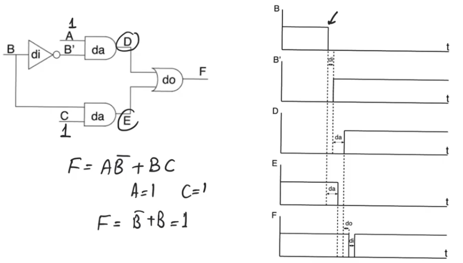
We can make the handoff numerical. Assume an idealized model in which the inverter, each AND gate, and the OR gate each delay a transition by exactly $1\mathrm{ns}$, and let $B$ fall at $t=0$. The lower AND output $BC$ falls at $t=1\mathrm{ns}$. The inverter’s output rises at $t=1\mathrm{ns}$, but the upper AND output $A\overline{B}$ does not rise until $t=2\mathrm{ns}$. Thus both OR inputs are low between those times. Accounting for the OR gate’s delay, $F$ falls at $t=2\mathrm{ns}$ and returns high at $t=3\mathrm{ns}$.

This fixed-delay illustration shows how a pulse can arise; ordinary $t_{\mathrm{PD}}$ bounds alone do not promise that particular pulse width, or even that a visible pulse will occur. Actual delays vary, and a sufficiently short internal pulse may not propagate through a gate. The defensible conclusions are that the unequal routes create a potential glitch and that the maximum path-delay bound tells us when the output must have settled.

What to do with a potential glitch

For the example above, the short $B$-to-$F$ route contains an AND and an OR; the longer route contains an inverter, an AND, and an OR. Spotting that reconvergence—one changing input influencing the same output through paths of different lengths—is a useful warning sign. It does not mean every input transition will glitch: here the concern is specifically the handoff with $A=C=1$ as $B$ falls.

One common response is timing discipline: allow the combinational network to settle, and use its output only after the maximum propagation-delay bound has elapsed. This is why a transient in a combinational datapath can be acceptable when its value is captured only at an appropriately timed sampling instant. A glitch is much more concerning if the output is used as an event signal, such as a clock, where even a brief pulse could be acted upon.

For this particular static-1 hazard, there is also a logic remedy. Add a term that remains high throughout the handoff:

The $AC$ term is redundant for the truth table: it does not change the settled Boolean function. Yet while $A=C=1$, it supplies a continuous reason for $F$ to stay high as $B$ changes. This illustrates a practical trade-off: minimum gate count and robust behavior during transitions are not always the same objective. Adding such a term addresses this single-input static hazard in the described implementation; it is not a blanket guarantee against glitches during arbitrary simultaneous input changes.

Watch the short follow-up for the two practical responses—waiting for settling and adding covering logic—and for why merely trying to match path delays is fragile.

Key takeaways

A combinational path’s propagation delay is a latest-settling bound: sum the maximum component delays along each path and use the largest total. Contamination delay is an earliest-disturbance bound: sum the minimum delays and use the smallest total. Neither tells you the exact instant a gate switches.

When a changing input reaches an output by reconverging routes, unequal delays can cause a glitch even if the initial and final truth-table values agree. Trace the intermediate terms to identify the risk, then decide whether the design can safely wait for settling or needs logic that holds the output through the transition.

Next, you’ll read timing diagrams more systematically, using the same input, internal-node, and output relationships to determine a combinational circuit’s behavior over time.