Interpreting Timing Diagrams in Combinational Circuits

Recommended resources

The freely available resources this lesson will direct you to.

Hello! Last lesson, you calculated how long a combinational path can take to settle and saw why unequal paths can produce a glitch. This lesson puts those ideas to work on timing diagrams: you’ll read input waveforms, determine what each gate sees over time, and explain when an output changes—or why an input change produces no output change at all.

The skill matters beyond hand-drawn circuits. Later, when you inspect simulated RTL waveforms, the same habit of tracing an output change back through its inputs will help you distinguish correct behavior from a timing or logic error.

Read a waveform as a series of intervals

A timing diagram has a shared horizontal time axis. Each signal occupies its own row: a high line represents logic 1, a low line represents logic 0, and a vertical edge marks a change. To determine a combinational output, divide the diagram at the input edges and ask what values the gate inputs have between edges.

Suppose $F = A \land B$ . If $A$ rises while $B = 0$ , $F$ stays low. If $B$ subsequently rises while $A = 1$ , the settled value of $F$ becomes high. The important distinction is that an input event is not necessarily an output event: an AND gate cannot respond visibly to a change that leaves at least one input low.

Watch the final example in Timing Diagrams (Digital Logic Tutorial) by Hydroxy The Tutor. Unlike a truth table with evenly spaced cases, its inputs change at irregular points. Focus on how the presenter reads each interval from the input traces rather than assuming every vertical line must cause an output edge.

Timing Diagrams (Digital Logic Tutorial) - Truth Table, Boolean expression as a Waveform, Explained

Watch the irregularly spaced input-waveform example to establish a reliable way of reading a combinational timing diagram.

Watch the waveform example. Locate each interval where both AND inputs are high, then notice the intervals where one input changes but the output's logical value does not. This example treats the gate as having no stated delay; we will add delay next.

For an ideal, zero-delay diagram, you can evaluate $F$ immediately on either side of every input edge. For a circuit with stated delays, keep that logical result separate from the time at which the output can reflect it. An intermediate signal is especially useful: first determine when that signal changes, then treat its waveform as an input to the next gate.

Follow the events through two gates

Consider an OR gate feeding an AND gate:

V = W \lor X, Z = Y \land V .

Assume for this worked diagram that each gate's output transition is drawn exactly $5 ns$ after the input condition that causes it. This is a convenient waveform-drawing model, not a general interpretation of a physical gate’s propagation-delay specification.

The image shows the circuit and its hand-drawn input traces. Use the circuit connections and time markings as your starting point; check any drawn output edges against the stated gate delays rather than taking a sketch as the timing rule.

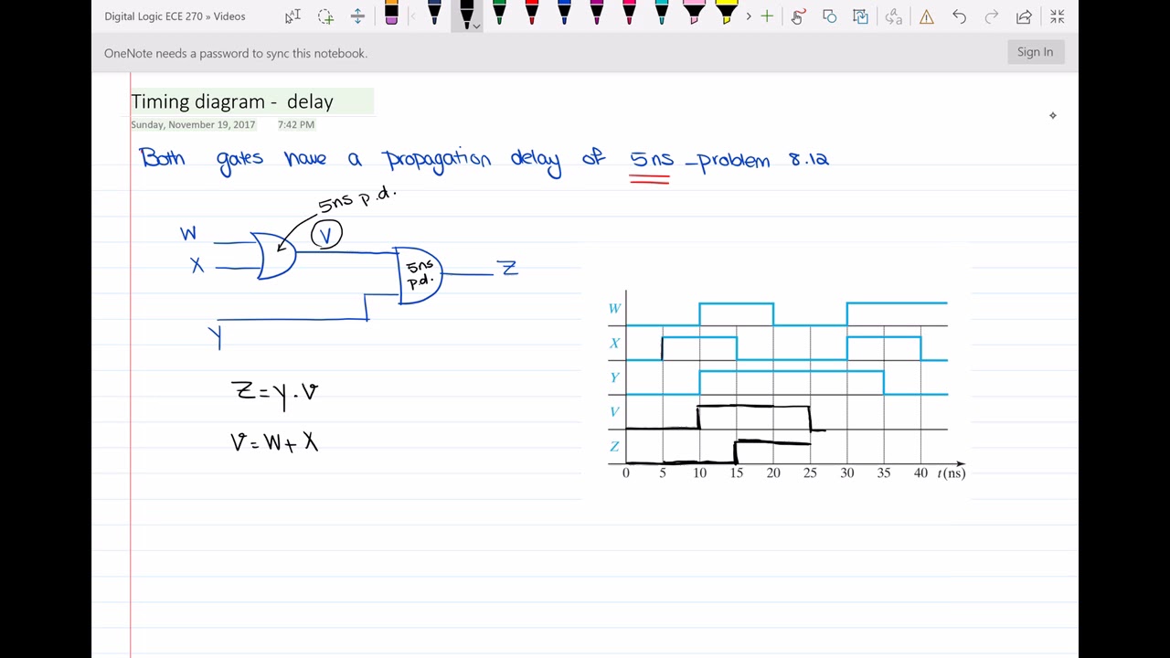
An OR gate produces intermediate signal $V$ from $W$ and $X$; an AND gate combines $V$ with $Y$ to produce $Z$. The input traces and 5 ns gate-delay assumption let us calculate the internal and output edge times.

Watch Timing diagram of the circuit with propagation delay from Electrical Engineering Authority for the gate-by-gate walkthrough. Pay particular attention to the distinction between the time an input changes and the time the affected gate output changes.

Timing diagram of the circuit with propagation delay

Watch the two-gate timing-diagram walkthrough to see how an internal waveform is used to determine the final output.

Begin with the setup for the circuit equations and initial levels. In the first edges, follow the change on X to V, then the change at the AND inputs to Z. Watch the falling edges for an input change that leaves V high and a later one that does not. Finish with the final inputs, checking why Z stays low when V becomes high again.

Here is the event trace under the stated exact-5-ns drawing assumption. Initially $W = X = Y = 0$ , so $V = Z = 0$ .

Time	Input event	Consequence for $V$ and $Z$
$5 ns$	$X$ rises	$V$ is scheduled to rise at $10 ns$ .
$10 ns$	$W$ and $Y$ rise; $V$ rises	Now $Y = V = 1$ , so $Z$ rises at $15 ns$ .
$15 ns$	$X$ falls; $Z$ rises	$W = 1$ still holds $V$ high; there is no new $V$ edge.
$20 ns$	$W$ falls	With $X = 0$ , $V$ falls at $25 ns$ .
$25 ns$	$V$ falls	$Y = 1$ , so $Z$ falls at $30 ns$ .
$30 ns$	$W$ and $X$ rise; $Z$ falls	$V$ rises at $35 ns$ .
$35 ns$	$Y$ falls; $V$ rises	$Z$ remains low because $Y = 0$ .

There are two easily missed moments here. At $15 ns$ , $X$ falls, but $W$ keeps the OR output high. At $25 ns$ , $V$ falls while $Y$ is high, so the AND output will fall—but not until $30 ns$ . If a hand-drawn $Z$ trace appears to fall at $25 ns$ , it has omitted the AND gate’s additional $5 ns$ in this model.

At $35 ns$ , the newly high $V$ does not make $Z$ high: $Y$ falls at that time. In the idealized trace, there is no interval in which both AND inputs are high again. In a physical implementation, the relative arrival times of those two edges would matter when assessing whether a brief pulse is possible; their coincidence on a sketch alone is not proof of glitch-free hardware.

Use intermediate traces to explain an observed output

Timing diagrams are also read in the other direction. When an output changes, locate the preceding input or intermediate-node edge that can explain it. The following image shows a larger circuit with two branches:

ab = a \land b, n c = c, x = ab \lor n c .

The AND and inverter branches produce $ab$ and $nc$, which meet at the OR gate producing $x$. The aligned traces let you explain each output interval from the two intermediate signals; no numerical gate-delay scale is supplied.

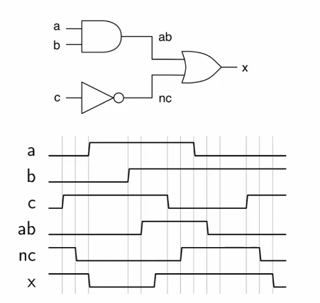
The separate $ab$ and $n c$ rows save you from mentally recomputing the entire expression at every edge. Near the start, $n c$ is high, so it holds $x$ high even though $ab$ is low. After $n c$ falls, both OR inputs are low and $x$ falls. Later, $ab$ rises and brings $x$ high. When $ab$ subsequently falls, $n c$ is already high, so $x$ does not fall. Near the end, $n c$ falls while $ab$ is low, allowing $x$ to fall again.

Notice the different kinds of conclusions available from this image. You can identify the order of visible events and which branch supports $x$ in each interval. You cannot assign a delay in nanoseconds to either branch from this diagram alone: its vertical guides do not supply a numerical time scale or gate-delay specification.

This gives you a compact method for interpreting an unfamiliar combinational waveform:

Read the circuit equation and identify useful intermediate nodes.
Mark the input-edge times, then determine the logic values between those times.
Explain or derive each intermediate trace using its own gate.
Explain the output from its immediate inputs, including periods when an input changes but the output does not.
Check what timing model is given. Use exact edge offsets only when the problem states that model; otherwise, distinguish observed edges from guaranteed settling bounds.

That last check connects directly to the previous lesson. A maximum propagation delay tells you when a result is guaranteed to have settled; it does not, by itself, specify the exact vertical edge you should draw. Nor does a settled Boolean expression rule out a transient between the old and new stable values.

Key takeaways

A timing diagram is a record of values over intervals, not just a collection of edges. For each gate, look at its immediate inputs and ask both whether their new values change its logical output and when the chosen timing model allows that change to appear. Intermediate traces make multi-gate behavior easier to follow, while unchanged outputs are often as informative as changing ones.

You have now completed the combinational-logic foundations. Next, the course moves to sequential circuits, where a further question becomes central: not just what value a circuit produces over time, but when a latch or flip-flop observes and retains it.