Degrees of Freedom Analysis: Mobility Equations

Hello! Welcome to the second module of our course, "Engineering Workflow and System Design."

In our last lesson, we set up a professional folder structure and discussed how to organize project documentation. This laid the groundwork for a systematic engineering process. Now, we'll dive into the first technical step of that process: analyzing the fundamental kinematics of a mechanism.

Today's lesson addresses the learning outcome: Apply mobility equations to evaluate degrees of freedom in a mechanism. Before we can design or select a mechanism for our linear actuator, we need a way to mathematically verify that a proposed design can move in the way we intend. This analysis, often called mobility or degree-of-freedom (DOF) analysis, is the first gate a concept must pass through. It ensures we don't waste time developing a mechanism that is locked up like a solid structure or one that moves uncontrollably.

1. What are Degrees of Freedom (DOF)?

Intuitively, the degrees of freedom (DOF) or mobility of a mechanism is the number of independent inputs required to fully define its position. For most simple machines driven by a single motor or handle, we want the mobility to be one.

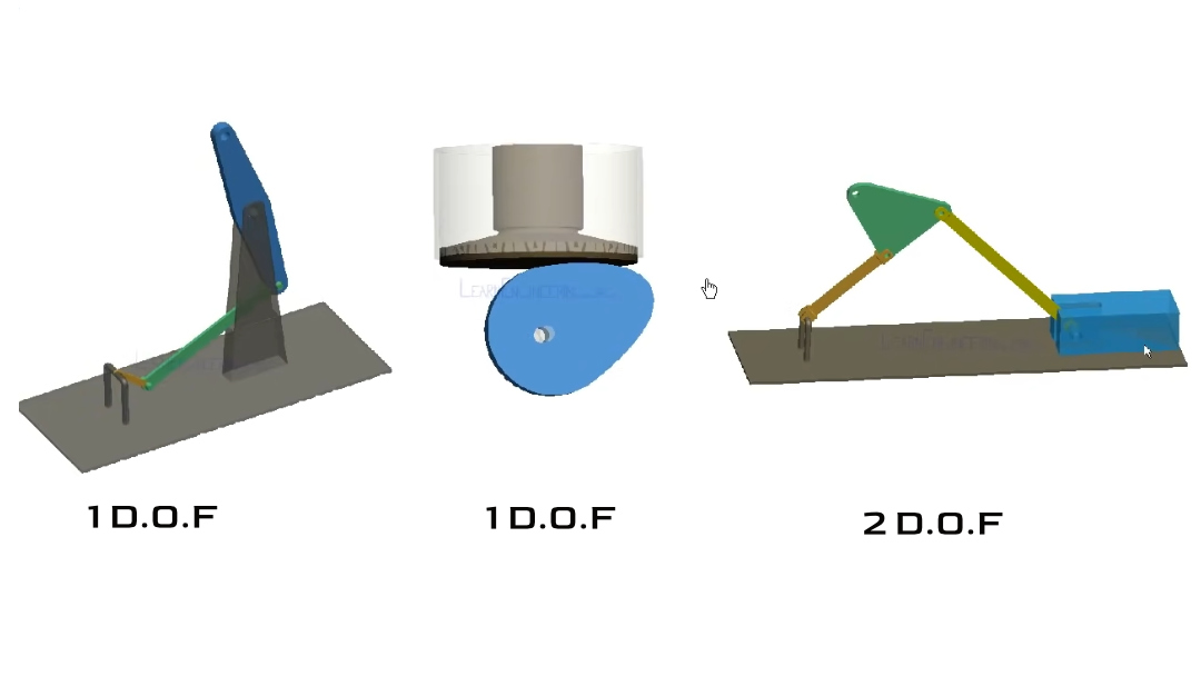
Comparing Degrees of Freedom in Mechanical Systems — This image illustrates the concept of mobility. The four-bar linkage and cam-follower on the left and in the center each have one degree of freedom (1-DOF), meaning the motion of a single input link controls the entire system. The more complex linkage on the right has two degrees of freedom (2-DOF), requiring two separate inputs to define its position.

For a mechanical engineer, this concept is formalized:

A rigid body free in a 2D plane has 3 DOF: translation along the x-axis, translation along the y-axis, and rotation about the z-axis.
A mechanism is a collection of rigid bodies (called links) connected by joints.
Joints introduce constraints, removing degrees of freedom.

The mobility (M) of the entire mechanism is the total possible DOF of all its moving links minus the constraints imposed by all its joints.

2. The Kutzbach Criterion for Planar Mechanisms

For planar (2D) mechanisms, the most common tool for calculating mobility is the Kutzbach criterion. It provides a simple formula to count up the freedoms and constraints.

To get a clear, intuitive explanation of this formula and see it in action, please watch the first part of the following video.

Mobility of Planar Mechanisms – Degrees of Freedom using Kutzbach Criterion

This video by Brian Bernard provides an excellent and practical introduction to the mobility equation, also known as the Kutzbach Criterion. It explains each term in the equation and then applies it to a real example.

Please watch from the beginning to 06:42. Focus on understanding: The meaning of each term in the mobility equation. The difference between j1 (lower pair) and j2 (upper pair) joints. The interpretation of the final mobility value (M=1, M>1, M=0, M<0).

Summarizing the Kutzbach Criterion

As the video explained, the equation is:
$M = 3 (n - 1) - 2 j_{1} - j_{2}$
Where:

M is the mobility or degrees of freedom of the mechanism.
n is the total number of links, including the stationary or "ground" link.
$j_{1}$ is the number of full joints (or lower pairs), which permit one degree of freedom and constrain two. Pin joints and sliders are the most common examples.
$j_{2}$ is the number of half joints (or higher pairs), which permit two degrees of freedom and constrain one. Examples include a wheel rolling on a surface or a cam-follower joint.

Interpreting the Result

M = 1: The mechanism is constrained and requires one input to control its motion. This is the goal for most single-actuator machines.
M = 0: The mechanism is a statically determinate structure. It cannot move.
M < 0: The mechanism is a statically indeterminate (or redundant) structure. It's locked and has extra constraints.
M > 1: The mechanism has more than one degree of freedom. It requires M independent inputs to be fully controlled.

3. Applying the Equation: Key Details and Examples

Counting links and joints seems straightforward, but there are a few common pitfalls. Let's formalize the process with some examples from a standard textbook.

kinematics, dynamics, and design of machinery

The textbook 'Kinematics, Dynamics, and Design of Machinery' offers formal definitions and clear, worked examples that will solidify your understanding. We'll focus on the section that introduces the mobility equation and applies it to several linkages.

Please read the section '1.7 CONSTRAINT ANALYSIS' (starts on page 12) up to the end of Example 1.3 on page 14. Pay special attention to: The formal definitions of Mobility and Connectivity. Example 1.1: A simple four-bar linkage. Example 1.3: How to count joints when more than two links connect at a single point.

Key Counting Rules:

The Ground Link: Always count the fixed frame or ground as one link (often labeled link #1), no matter how many separate grounded points are shown in a diagram. All fixed points are part of the same rigid body.
Multi-Link Joints: A single pin connecting p links must be counted as p-1 joints. For instance, if three links are pinned together at one spot, that counts as $3 - 1 = 2$ pin joints for our calculation. This was shown in Example 1.3 from the reading.

Test your understanding!

Let's apply this to the mechanism in the image below. This is problem 1.22(d) from a textbook. The pin-in-slot joint allows both rotation and sliding, so it is a full joint ( $j_{1}$ ) because the pin is fully captured in the slot. The rolling contact is a half joint ( $j_{2}$ ).

Mechanism Mobility Analysis Examples — Focus on problem (d) at the bottom left. Calculate its mobility using the Kutzbach criterion.

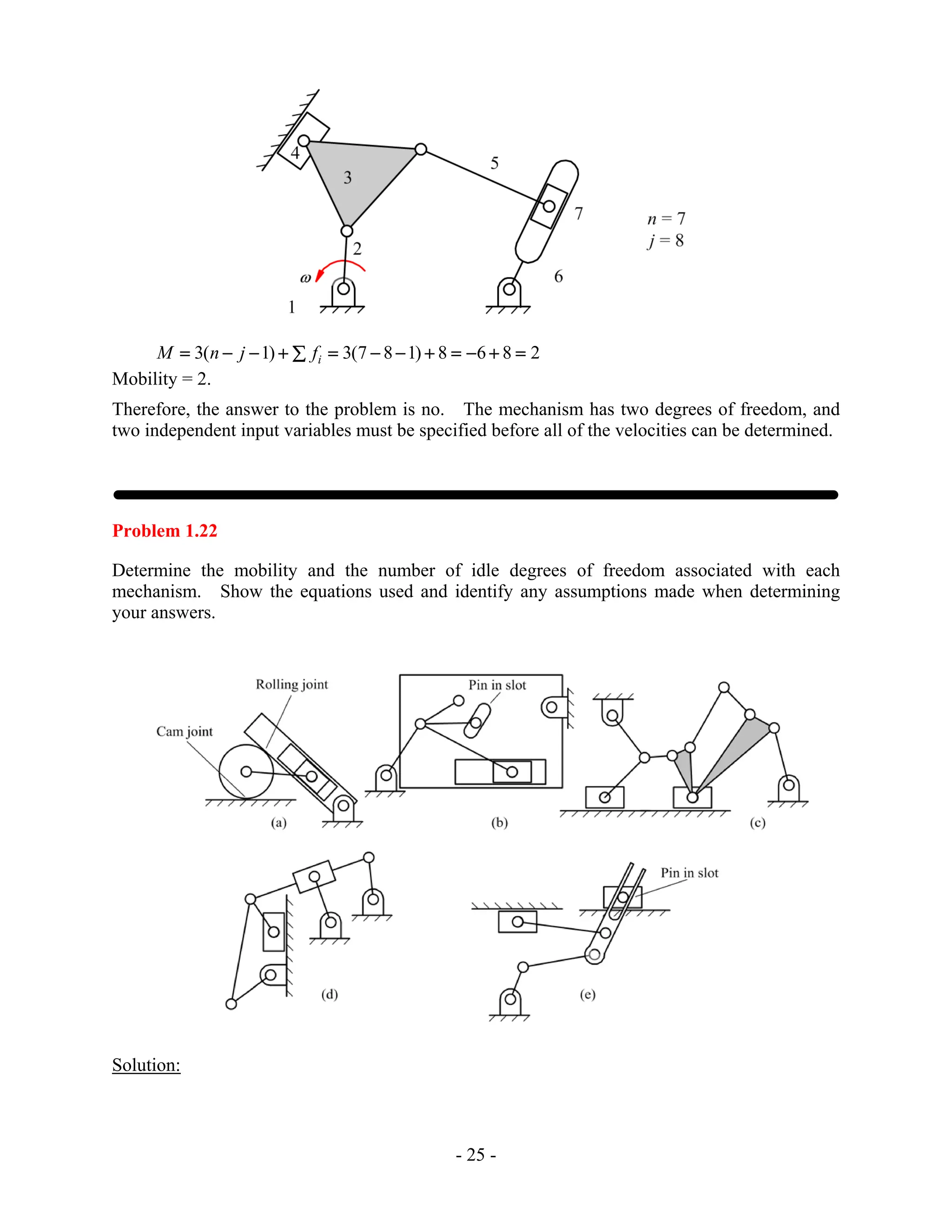
How many links (n), full joints ( $j_{1}$ ), and half joints ( $j_{2}$ ) do you count? What is the resulting mobility (M)?

Show answer

Links (n): There are 4 links.
1. The ground (the fixed surface and the fixed pin joint center).
2. The vertical link with the slot.
3. The link connecting the pin and the roller.
4. The roller itself.
  So, n = 4.
Full Joints ( $j_{1}$ ): There are 3 full joints.
1. The pin joint connecting the slotted link to the ground.
2. The pin joint connecting the roller link to the slotted link (this is the pin-in-slot).
3. The pin joint connecting the roller to its link.
  So, $j_{1}$ = 3.
Half Joints ( $j_{2}$ ): There is 1 half joint.
1. The rolling contact between the roller and the ground.
  So, $j_{2}$ = 1.
Mobility Calculation:
$M = 3 (n - 1) - 2 j_{1} - j_{2}$
$M = 3 (4 - 1) - 2 (3) - 1$
$M = 3 (3) - 6 - 1$
$M = 9 - 6 - 1 = 2$

The mobility of this mechanism is M = 2. This means you would need two independent inputs to control its position.

4. A Note on 3D (Spatial) Mechanisms

The Kutzbach criterion we've been using is for planar mechanisms. For spatial (3D) mechanisms, the principle is the same, but the numbers change. A rigid body free in space has 6 DOF (translation in x, y, z and rotation about x, y, z). The mobility equation becomes:

$M = 6 (n - 1) - \sum_{i = 1}^{j} (6 - f_{i})$

Where:

n is the number of links.
j is the number of joints.
$f_{i}$ is the degrees of freedom (or connectivity) of the i-th joint. For example, a simple pin or revolute joint in 3D still only allows 1 DOF ( $f = 1$ ). A ball-and-socket joint allows 3 DOF ( $f = 3$ ).

A famous example of a spatial mechanism is the Stewart Platform, which uses 6 linear actuators to achieve 6-DOF motion. Calculating its mobility requires this 3D formula. While we won't delve into spatial analysis in this course, it's valuable to know that the fundamental concept of counting freedoms and constraints extends to three dimensions.

Conclusion

Today, we've added a fundamental analytical tool to our engineering workflow. By applying the mobility equation, we can quickly validate whether a mechanism concept is kinematically sound before investing time in detailed design and CAD modeling.

Key Takeaways:

The mobility (M) or degrees of freedom (DOF) of a mechanism determines the number of independent inputs needed to control it. For most single-actuator designs, the goal is M=1.
The Kutzbach criterion ( $M = 3 (n - 1) - 2 j_{1} - j_{2}$ ) is a simple and powerful tool for calculating the mobility of planar mechanisms.
Accurate counting is crucial: remember to count the ground as one link and to properly account for multi-link joints ( $p$ links = $p - 1$ joints).
The concept extends to 3D mechanisms, where the base number for DOF is 6 instead of 3.

In our next lesson, we will move from analyzing mobility to choosing a mechanism type. We will explore different kinds of mechanisms (like linkages, cams, and sliders) and discuss how to select the most appropriate one to meet the motion requirements we defined for our linear actuator project. The mobility calculation will be our first check for any concept we consider.

Recommended resources