Hello! Welcome to your next lesson in our "Shortest Paths and Minimum Spanning Trees" module.
In the last lesson, you mastered Dijkstra's algorithm, a fast and efficient way to find the shortest paths from a single source. We ended with a crucial cliffhanger: Dijkstra's algorithm relies on a greedy approach that only works if all edge weights are non-negative.
Today, we will address that limitation directly. Your learning goal is to describe the use cases for the Bellman-Ford algorithm, which is specifically designed for graphs that may contain negative edge weights. Understanding when and why to use Bellman-Ford is a key piece of knowledge for tackling a wider range of graph problems in competitive programming.
We'll cover:
- Why Dijkstra's algorithm fails with negative weights.
- The core mechanism of the Bellman-Ford algorithm.
- How Bellman-Ford's unique structure allows it to detect "negative cycles," a critical concept in many problems.
1. The Problem with Negative Weights
Dijkstra's algorithm is greedy. It finalizes the path to the closest unvisited node at each step, assuming that no shorter path will ever be found. A negative edge can break this fundamental assumption.
Consider a simple path: A -> B has a weight of 5. Dijkstra's might explore from A, find B, and declare its shortest distance as 5. But what if there's another path A -> C -> B, with weights A->C (10) and C->B (-6)? The total path weight is 4, which is shorter. If Dijkstra's already finalized node A and moved on, it might miss this better path to B.
This is where Bellman-Ford comes in. It's a more methodical, less "optimistic" algorithm.

2. The Bellman-Ford Approach: Relaxing Every Edge
Unlike Dijkstra's which uses a priority queue to greedily pick the next best node, Bellman-Ford takes a more exhaustive approach based on dynamic programming. The core idea is simple but powerful:
Relax every single edge in the graph V-1 times, where V is the number of vertices.
A "relaxation" is the same step you saw in Dijkstra's:if distance[u] + weight(u, v) < distance[v]:distance[v] = distance[u] + weight(u, v)
Why V-1 times? In a graph with no negative cycles, the longest possible shortest path can have at most V-1 edges. By iterating V-1 times, the algorithm ensures that the shortest path distances have propagated all the way across the graph, even in the worst-case scenario (like a long, straight-line graph).
To get a deep intuition for this V-1 rule, watch this excellent explanation.
The video 'G-41. Bellman Ford Algorithm' from the popular competitive programming channel 'take U forward' provides a brilliant, intuitive reason for the V-1 iterations. This is a key insight that many tutorials gloss over.
Watch from 04:55 to 07:08 to understand the relaxation concept, and then from 14:44 to 21:13 for the core intuition. Focus on how the worst-case graph (a long chain) demonstrates why exactly V-1 iterations are necessary to guarantee the shortest path is found.
3. Use Case 1: Finding Shortest Paths with Negative Edges
The most direct use case for Bellman-Ford is to solve the single-source shortest path problem when negative edge weights are present (but there are no negative cycles).
Think of a scenario where edges represent transactions:
- A positive weight could be a cost or travel time.
- A negative weight could represent a profit, a discount, or a "boost" you gain by taking that path.
The Medium article "Dijkstra's vs Bellman-Ford Algorithm" provides a simple, practical example using airline routes with a discount.
Dijkstra's vs Bellman-Ford Algorithm
Let's read a short section of this article to see a concrete example of a negative weight in action.
Read the section 'Using Bellman-Ford Algorithm'. It starts by introducing a negative edge weight for an airline discount and shows the table of distances being updated. You don't need to trace every number, just grasp how the negative weight influences the final shortest path.
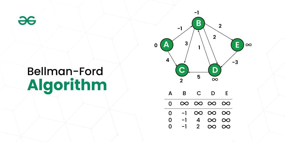
4. Use Case 2: Detecting Negative Cycles
This is arguably the most important and unique feature of the Bellman-Ford algorithm. What happens if there's a cycle of edges whose weights sum to a negative number?
If you traverse such a cycle, your total path cost decreases. You could go around it again and decrease the cost further... and again, and again, infinitely. In this case, the "shortest path" to any node reachable from the cycle is negative infinity.
Dijkstra's algorithm would get stuck in an infinite loop. Bellman-Ford, however, can elegantly detect this situation.
How it works:
- Run the main algorithm for
V-1iterations. This finds the shortest paths if no negative cycles exist. - Perform one more iteration (the
Vthiteration). - If any distance value can still be improved during this
Vthpass, it means that node is part of, or reachable from, a negative cycle.
This detection capability is a powerful tool. A classic application is in finance, for detecting arbitrage opportunities. Imagine currencies are nodes and exchange rates are edges. A negative cycle means you can convert money through a series of currencies and end up with more than you started with—a risk-free profit.
This video provides a great overview of negative cycles and their detection.
Bellman Ford Algorithm | Shortest path & Negative cycles | Graph Theory
The video 'Bellman Ford Algorithm | Shortest path & Negative cycles' by WilliamFiset clearly explains what negative cycles are and their practical implications.
Watch from the beginning to 04:00. Pay close attention to: The comparison with Dijkstra's (0:00-1:34). The arbitrage example (1:34-1:59). The visual explanation of how a negative cycle makes reachable paths go to negative infinity (1:59-4:00). The brief mention of how the algorithm is run a 'second time' to detect these cycles.
Test your understanding!
Imagine you're running Bellman-Ford on a graph with 5 vertices (V=5). You complete the required V-1 = 4 iterations and have your final distances array. Now, you perform the 5th iteration to check for negative cycles. During this 5th pass, you are relaxing the edge A -> B with weight -2, and you find that distance[A] + (-2) is less than the current distance[B]. What can you conclude?
Show answer
You can conclude that a negative cycle exists in the graph, and that node B is either part of that cycle or is reachable from it. The shortest path to B is technically negative infinity, as you could keep traversing the cycle to lower its cost indefinitely.
5. Summary: Bellman-Ford vs. Dijkstra
So, when do you use each algorithm? The choice depends entirely on the constraints of the problem, specifically the edge weights.
| Feature | Dijkstra's Algorithm | Bellman-Ford Algorithm |
|---|---|---|
| Edge Weights | Only non-negative | Can handle negative weights |
| Negative Cycles | Fails (may enter an infinite loop) | Detects them and can report their existence |
| Approach | Greedy (uses a priority queue) | Dynamic Programming (iteratively relaxes all edges) |
| Time Complexity | O(E log V) or O((E+V)logV) (with a priority queue) |
O(V * E) |
| Primary Use | The default, faster choice for general SSSP problems. | When graph has negative edges, or when you need to check for negative cycles. |
Because of its higher time complexity, you should prefer Dijkstra's if you are certain there are no negative edges. If the problem allows for negative edges or asks you to detect a negative cycle, Bellman-Ford is your tool.
Conclusion
In this lesson, you've learned about the specific and powerful use cases for the Bellman-Ford algorithm. It serves as a more robust, albeit slower, alternative to Dijkstra's when graphs get more complex.
Key Takeaways:
- Bellman-Ford's main use case is finding single-source shortest paths in graphs with negative edge weights.
- Its second, equally important use case is detecting negative cycles, which represent situations where a path's cost can be infinitely reduced.
- The algorithm works by relaxing all edges
V-1times. AVthrelaxation pass is used to identify nodes affected by negative cycles. - It is slower (
O(V*E)) than Dijkstra's, so you should only use it when necessary.
Up Next:
We are now going to switch gears from shortest path problems. In the next lesson, we will introduce a completely new data structure: the Disjoint Set Union (DSU). It's an incredibly efficient tool for solving problems related to connectivity and partitioning sets, and it will be our foundation for learning about Minimum Spanning Trees.