Dijkstra's Algorithm with Priority Queues

1. The Shortest Path Problem

Imagine a road network where cities are nodes and roads are edges, each with a weight representing the travel time. The goal is to find the fastest route from a starting city to all other cities. This is the essence of the single-source shortest path problem.

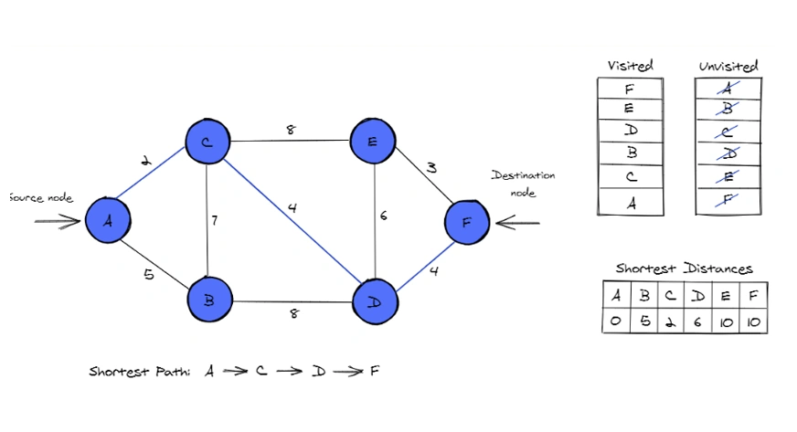
Dijkstra's algorithm solves this problem using a greedy strategy. At each step, it visits the unvisited node that has the smallest known distance from the start node. It's like always choosing the next closest city to explore from your current set of options.

To understand this greedy approach visually, let's watch a detailed walkthrough.

2. The Core Components of Dijkstra's Algorithm

As you saw in the video, the algorithm maintains a few key pieces of information:

1. A distances data structure: This stores the shortest distance found so far from the source node to every other node. It's typically an array or dictionary, initialized with infinity for all nodes except the source, which is 0.
2. A set of visited nodes: To avoid processing a node more than once and getting into cycles. Once we finalize the shortest path to a node, we add it to this set.
3. A priority queue: This is the crucial component for efficiency. It stores (distance, node) pairs and always allows us to quickly retrieve the unvisited node with the smallest current distance. This is exactly what the heapq module you learned about in Module 8 is for.

3. Why Use a Priority Queue?

The video mentioned that using a priority queue is a critical optimization. Let's make that concrete.

Without a priority queue, at every step of the algorithm, you would have to scan through the entire distances array to find the unvisited node with the minimum distance. This would take $O(V)$ time for each of the $V$ vertices, leading to a total time complexity of $O(V^2)$.

By using a min-heap (our priority queue), we can get the next closest node in $O(\log V)$ time. This simple change dramatically improves the algorithm's performance.

4. Implementing Dijkstra's Algorithm in Python

Now, let's translate this logic into a clean Python implementation. For competitive programming, you want a template that is both correct and quick to write.

Let's watch a walkthrough of a typical implementation. This will help you connect the conceptual steps to actual code.

The video shows the complete logic. Let's formalize that into a standard template you can use. This template is very similar to the one found in the coderraj07 article.

The Python Template

Here is a well-commented template for Dijkstra's algorithm.

import heapq

def dijkstra(n, edges, start_node):
    # 1. Represent the graph using an adjacency list (dictionary in this case)
    adj = {i: [] for i in range(n)}
    for u, v, weight in edges:
        adj[u].append((v, weight))
    
    # 2. Initialize distances to all nodes as infinity
    distances = {i: float('inf') for i in range(n)}
    distances[start_node] = 0
    
    # 3. Initialize the priority queue (min-heap) with the start node
    # The heap stores tuples of (distance, node)
    min_heap = [(0, start_node)]
    
    while min_heap:
        # 4. Pop the node with the smallest distance from the heap
        current_dist, current_node = heapq.heappop(min_heap)
        
        # 5. IMPORTANT: If we've found a shorter path already, skip
        # This handles "stale" entries in the heap
        if current_dist > distances[current_node]:
            continue
            
        # 6. Explore neighbors (Relaxation step)
        for neighbor_node, weight in adj[current_node]:
            new_dist = current_dist + weight
            
            # 7. If we found a shorter path to the neighbor, update it
            if new_dist < distances[neighbor_node]:
                distances[neighbor_node] = new_dist
                # 8. Push the updated distance and neighbor to the heap
                heapq.heappush(min_heap, (new_dist, neighbor_node))
                
    # Post-processing: Mark unreachable nodes if required by the problem
    for i in range(n):
        if distances[i] == float('inf'):
            distances[i] = -1 # Or whatever the problem specifies
            
    return distances

# Example Usage:
# n = number of nodes
# edges = list of [source, destination, weight]
# start_node = the node to start from

n = 6
edges = [[0, 1, 7], [0, 2, 9], [0, 5, 14], [1, 2, 10], [1, 3, 15], 
         [2, 3, 11], [2, 5, 2], [3, 4, 6], [4, 5, 9]]
start_node = 0

shortest_paths = dijkstra(n, edges, start_node)
print(f"Shortest paths from node {start_node}: {shortest_paths}")
# Expected output: {0: 0, 1: 7, 2: 9, 3: 20, 4: 26, 5: 11}

The check if current_dist > distances[current_node]: continue is a crucial optimization. When we find a shorter path to a node, we push the new, shorter path to the heap. We don't remove the old, longer path entry. This check ensures we only process a node the first time we pull its true shortest path from the heap.

Conclusion

Congratulations! You have now learned how to implement one of the most essential graph algorithms for competitive programming.

Key Takeaways:

• Dijkstra's algorithm finds the single-source shortest paths in a weighted graph with non-negative edge weights.
• It operates on a greedy principle, always exploring from the unvisited node that is currently closest to the source.
• Using a min-heap (priority queue) is critical for an efficient implementation, achieving a time complexity of $O((E+V)\log V)$.
• The core logic involves initializing distances, using a while loop that pops from the heap, and performing the relaxation step for all neighbors.

Up Next:
Dijkstra's algorithm has one major limitation: it does not work correctly if the graph contains negative edge weights. In our next lesson, we will explore the Bellman-Ford algorithm, which is designed to handle exactly that scenario.