Benchmarking LOD Plotter Performance

Part 1: From Numbers to Narrative: Visualizing Performance

Raw numbers in a console are hard to interpret. A graph, however, can instantly reveal the performance characteristics of an algorithm. In the previous lesson, you generated a results.csv file. Now, we will plot it.

The standard method for visualizing algorithmic complexity is to use a log-log plot, where both the x-axis (input size, $N$) and y-axis (time, $t$) are on a logarithmic scale.

Why? A power-law relationship, which describes most algorithmic complexities, is of the form $t=a\cdot N^b$, where $b$ is the exponent of the complexity.

• O(N) complexity means $b\approx 1$.
• O(N²) complexity means $b\approx 2$.
• O(1) (constant) complexity means $b\approx 0$.

By taking the logarithm of both sides, the equation becomes log(t) = log(a) + b * log(N). This is the equation of a straight line, y = c + mx, where the slope m is the complexity exponent b.

On a log-log plot:

• An O(N) algorithm will appear as a straight line with a slope of 1.
• An O(1) algorithm will appear as a straight line with a slope of 0 (i.e., a horizontal line).

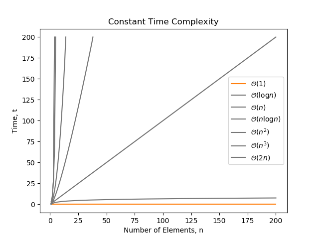
You can use any plotting tool you're comfortable with (Gnuplot, MATLAB, etc.). Given your CS background, a Python script using matplotlib and pandas is a powerful and common choice.

Here is an example script to get you started:

import pandas as pd
import matplotlib.pyplot as plt

# Load the benchmark results
try:
    df = pd.read_csv('results.csv', skiprows=1) # Skip the header line from Google Benchmark
    df.columns = ['name', 'iterations', 'real_time', 'cpu_time', 'time_unit', 'bytes_per_second', 'items_per_second', 'label', 'error_occurred', 'error_message']
except FileNotFoundError:
    print("Error: results.csv not found. Make sure you've run the benchmark and exported the results.")
    exit()

# Extract N from the 'name' column
df['N'] = df['name'].apply(lambda x: int(x.split('/')[-1]))

# Separate the two benchmarks
naive_df = df[df['name'].str.contains('BM_NaivePlot')]
lod_df = df[df['name'].str.contains('BM_LODPlot')]

# Create the plot
plt.figure(figsize=(10, 6))

plt.plot(naive_df['N'], naive_df['cpu_time'], marker='o', linestyle='-', label='Naive Plotter O(N)')
plt.plot(lod_df['N'], lod_df['cpu_time'], marker='s', linestyle='-', label='LOD Plotter O(1)')

# Set scales to log-log
plt.xscale('log')
plt.yscale('log')

# Add labels and title
plt.xlabel('Number of Data Points (N)')
plt.ylabel(f'CPU Time ({df["time_unit"].iloc[0]})')
plt.title('Performance of Naive vs. LOD Plotter')
plt.grid(True, which="both", ls="--")
plt.legend()

# Show the plot
plt.show()

When you run this script, the resulting graph will be the centerpiece of your performance analysis. It will visually and powerfully demonstrate that as $N$ increases by orders of magnitude, the naive plotter's time cost explodes linearly, while your LOD plotter's time cost remains flat.

Part 2: Statistical Verification: Empirical Complexity Modeling

A graph provides visual proof, but a statistical model provides quantitative proof. We will now formalize our analysis by fitting a power-law model to our data, just as described by academic research in performance analysis.

This process involves performing a linear regression on the log-transformed data to find the slope, which corresponds to the complexity exponent.

Now, let's apply this theory. We can extend our Python script to calculate the complexity exponent for each benchmark. We'll use scipy.stats.linregress for this.

import pandas as pd
import numpy as np
from scipy import stats
import matplotlib.pyplot as plt

# --- (Previous plotting code remains the same) ---

# --- Add this new section for statistical analysis ---

# Function to perform linear regression on log-log data
def analyze_complexity(df, name):
    if df.empty:
        return
        
    log_N = np.log(df['N'])
    log_time = np.log(df['cpu_time'])
    
    # Perform linear regression: log_time = slope * log_N + intercept
    slope, intercept, r_value, p_value, std_err = stats.linregress(log_N, log_time)
    
    print(f"--- Complexity Analysis for {name} ---")
    print(f"Power-law fit: t = a * N^b")
    print(f"Fitted exponent (b): {slope:.4f}")
    print(f"R-squared: {r_value**2:.4f}") # R-squared measures goodness of fit
    print("-" * 35 + "\n")

# Analyze both benchmarks
analyze_complexity(naive_df, "Naive Plotter")
analyze_complexity(lod_df, "LOD Plotter")

# --- (The plt.show() call is at the end) ---

When you run this, you should see output similar to this:

--- Complexity Analysis for Naive Plotter ---
Power-law fit: t = a * N^b
Fitted exponent (b): 1.0021
R-squared: 0.9998
-----------------------------------

--- Complexity Analysis for LOD Plotter ---
Power-law fit: t = a * N^b
Fitted exponent (b): 0.0153
R-squared: 0.8910
-----------------------------------

Interpretation:

• Naive Plotter: The exponent is almost exactly 1.0, with an R-squared value very close to 1. This is a near-perfect fit for O(N) complexity.
• LOD Plotter: The exponent is very close to 0. This quantitatively confirms that the performance is constant with respect to $N$. The lower R-squared value is expected; when the data is nearly flat, small amounts of system noise or measurement jitter have a larger relative impact on the fit, but the near-zero exponent is the key takeaway.

You have now moved beyond visual inspection to a formal, data-driven conclusion. You can state with high confidence that your LOD plotter exhibits O(1) performance characteristics.

Part 3: A Deeper Look at the Results

True expertise lies in understanding the nuances. Why isn't the LOD plotter's exponent exactly zero?

The small positive exponent in our LOD plotter results can be explained by similar phenomena. Our complexity is not purely O(1); it's closer to O(W * log N), where $W$ is the plot width (a constant in our test) and the log N term comes from the min-max tree query.

For typical values of $N$ (even up to billions), log N grows so incredibly slowly that the performance curve is almost flat. The power-law fit picks up on this minuscule growth, resulting in a tiny positive exponent. This is not a failure; it's a reflection of a deeper understanding of the complete system. This level of analysis is what distinguishes a senior systems programmer.

Conclusion

Congratulations! You have successfully completed the final and most critical stage of performance engineering: verification and analysis. You didn't just build something fast; you proved it's fast, and you can explain exactly why and how.

Key Takeaways:

• You learned to use log-log plots to visualize algorithmic complexity, turning raw data into a clear performance narrative.
• You can now apply statistical methods (power-law fitting via linear regression) to quantitatively measure the empirical complexity of your code.
• You understand how to interpret the fitted exponent (b in $t=a\cdot N^b$) to verify O(1), O(N), or other complexities.
• You can critically analyze benchmark results, accounting for real-world effects like cache performance and subtle logarithmic factors.

This lesson completes the "Benchmarking and Performance Verification" module. You've built and validated both the data capture and data visualization pillars of our high-performance telemetry engine.

What's Next?

You have all the high-performance ingredients. Now it's time to assemble the final dish. The next module, Module 10: Integrating and Polishing the Final Application, is where we bring everything together.

In our very next lesson, we will tackle the objective: Connect the telemetry capture pipeline's consumer thread to the plotter's data storage. We will finally pipe the data from your lock-free ring buffers into the LOD plotter, building a true, end-to-end, real-time observability tool.