Profiling Plotter Performance

What is Profiling and Why Use Tracy?

It's important to distinguish between the two main tools for performance analysis:

• Benchmarking: Measures the performance of specific, isolated code paths under controlled conditions. We used Google Benchmark to measure the time taken by your render function for different input sizes (N). This is ideal for determining algorithmic complexity and making macro-level comparisons.
• Profiling: Traces the execution of an entire application as it runs, providing a detailed breakdown of where time is spent, how functions call each other, how threads interact, and how memory is used. It's the go-to tool for hunting down specific, unknown bottlenecks in a complex system.

For our project, Tracy Profiler is an excellent choice. It's a low-overhead, real-time frame profiler that gives you an interactive, graphical view of your application's performance.

As you read, notice that Tracy isn't just a profiler; it's a diagnostic tool that visualizes CPU cycles, memory allocations, and even lock contention, making it invaluable for the kind of systems you aim to build.

Part 1: Integrating Tracy into Your Project

Let's get our hands dirty and add Tracy to your plotter application. The process involves two main components: integrating the Tracy client into your C++ code and building the separate Tracy viewer application.

We will follow a clear guide for this process. The steps below assume you have a cmake project structure, which we've been using throughout the course.

Step-by-Step Integration

1. Clone the Tracy Repository:
   In your project's root directory, create a folder named external if you don't already have one. Then, clone Tracy into it:

   cd external
   git clone https://github.com/wolfpld/tracy.git
   cd ..
   

2. Update CMakeLists.txt:
   Modify your main CMakeLists.txt file to include the Tracy client. The changes below tell CMake where to find Tracy, enable its instrumentation, and link it to your executable.

   # Add this block to your CMakeLists.txt
   
   # --- Tracy Profiler Integration ---
   # Enable Tracy. When this is OFF, all Tracy macros become no-ops.
   option(TRACY_ENABLE "Enable Tracy Profiler" ON)
   
   if(TRACY_ENABLE)
       add_subdirectory(external/tracy)
       # For some Tracy versions/platforms, you might need to add this include directory
       # target_include_directories(your_executable_name PRIVATE external/tracy)
   endif()
   
   # In your target_link_libraries, add Tracy::TracyClient
   target_link_libraries(your_executable_name PRIVATE
       # ... your other libraries like ImGui, glad, glfw ...
       ${IMGUI_LIBS}
       ${GLAD_LIBS}
       ${GLFW_LIBS}
   )
   
   if(TRACY_ENABLE)
       target_link_libraries(your_executable_name PRIVATE Tracy::TracyClient)
   endif()
   

   Make sure to replace your_executable_name with the actual name of your project's target. The TRACY_ENABLE option is crucial: it allows you to completely compile out all profiling code for a final release build, ensuring zero overhead.

3. Build the Tracy Viewer:
   The viewer is a separate GUI application that receives and displays the data from your program.

   • First, install its dependencies (on a Debian/Ubuntu system):

     sudo apt install libglfw3-dev libfreetype-dev libcapstone-dev libdbus-1-dev
     

   • Then, navigate into the Tracy repository and build the viewer. The command depends on your display server (most modern Linux desktops use Wayland, but X11 is also common).

     cd external/tracy/profiler/build/unix
     # For Wayland (default):
     make
     # OR for X11:
     # make LEGACY=1
     cd ../../../../ # Return to your project root
     

   This will create an executable named Tracy-release inside external/tracy/profiler/build/unix.

4. Rebuild Your Application:
   Now, re-run CMake and build your project to link the Tracy client.

   cd build
   cmake ..
   make
   

Your application is now instrumented, but it isn't sending any data yet. For that, we need to add profiling "zones."

Part 2: Instrumenting Your Code with Profiling Zones

Tracy works by letting you mark specific blocks of code as "zones." When your program executes, Tracy records the entry and exit times of these zones, which allows it to build the call stack and flame graph.

The primary macro for this is ZoneScoped.

1. Include the Tracy Header: At the top of the .cpp file containing your main loop and plotter logic, add:

   #include "tracy/Tracy.hpp"
   

2. Mark Your Frames: In your main while loop, right at the end (after rendering and swapping buffers), add a FrameMark macro. This tells Tracy where one frame ends and the next begins, which is essential for analyzing frame times.

   // In your main loop
   while (!glfwWindowShouldClose(window)) {
       // ... poll events, start new ImGui frame ...
   
       // --- Your Plotter Rendering ---
       lod_plotter.render();
   
       // ... ImGui::Render(), display render data ...
   
       glfwSwapBuffers(window);
       
       // Add this line!
       FrameMark; 
   }
   

3. Instrument the Plotter: Let's add zones to the key parts of your LOD plotter to see where time is spent. This is the most critical step for our analysis.
   In your plotter's render function:

   void LODPlotter::render() {
       ZoneScoped; // This zone will be named "LODPlotter::render"
   
       // ... existing ImGui::Begin() code ...
   
       // Let's add more specific zones for deeper analysis
       {
           ZoneScopedN("Calculate Visible Range"); // A custom-named zone
           // ... your logic to calculate visible data range based on zoom/pan ...
       }
   
       {
           ZoneScopedN("Query Min-Max Tree & Decimate");
           // ... your loop that queries the tree and adds points/bars to a temporary buffer ...
       }
   
       {
           ZoneScopedN("Submit ImGui Draw Commands");
           ImDrawList* draw_list = ImGui::GetWindowDrawList();
           // ... your loop that iterates the temporary buffer and calls draw_list->AddLine() etc. ...
       }
       
       // ... existing ImGui::End() code ...
   }
   

   ZoneScoped automatically uses the function name as the zone name. ZoneScopedN("My Custom Name") lets you provide a more descriptive name, which is very useful for loops or logical blocks within a single function.

Part 3: Capturing and Analyzing Your First Profile

With the code instrumented, you're ready to see the results.

1. Run the Tracy Viewer:
   Open a terminal and launch the viewer you built earlier.

   ./external/tracy/profiler/build/unix/Tracy-release
   

   A window will appear, waiting for a connection.

2. Run Your Instrumented Application:
   In a separate terminal, run your plotter executable.

   ./build/your_executable_name
   

   Almost immediately, you should see your application appear in the Tracy viewer, and data will start streaming in.

3. Analyzing the Profile:
   Let the application run for a few seconds and then click the "Pause" button in the Tracy UI. Now you can inspect the captured data.

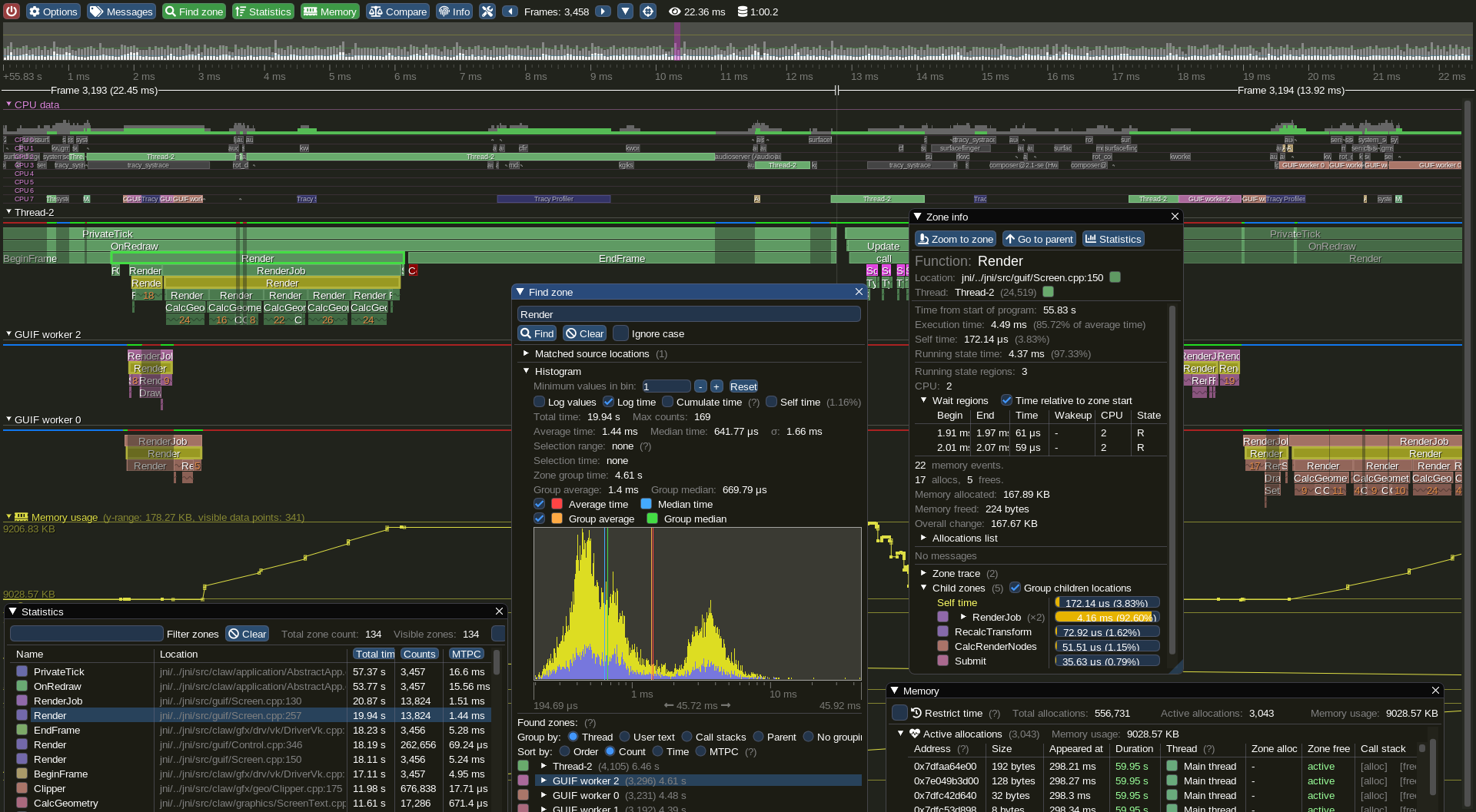
*This is a typical Tracy view. The main area is a timeline (flame graph) showing function calls over time across different threads. You can zoom, pan, and click on individual blocks ('zones') to get detailed statistics.*

Here's what to look for to analyze your plotter's performance:

*   **The Main Thread Timeline:** Find the main thread in the list on the left. You should see a repeating pattern of colored bars corresponding to each frame of your application.
*   **Find Your Zones:** Zoom in on a single frame (using the mouse wheel). You should be able to see the `LODPlotter::render` zone.
*   **Drill Down:** If you expand the `LODPlotter::render` zone, you will see the child zones we created: `Calculate Visible Range`, `Query Min-Max Tree & Decimate`, and `Submit ImGui Draw Commands`.
*   **Check Timings:** Click on the `LODPlotter::render` zone. A statistics panel will appear. It shows the total time, self time (time spent only in that function, excluding children), and other useful metrics.

*This view shows detailed statistics for a selected zone, including memory usage, call stack information, and timing distributions. This is where you can dig deep into a specific function's behavior.*

**The Core Question:** Where is the time being spent?
Based on our previous benchmarks, we expect the `Query Min-Max Tree & Decimate` zone to be extremely fast and take up a tiny fraction of the total render time. The majority of the time should be spent in `Submit ImGui Draw Commands`. Does your Tracy profile confirm this? By visually comparing the widths of these zones, you can immediately validate your understanding of the performance breakdown.

Conclusion and Your Next Steps

Congratulations! You have successfully used a professional-grade profiler to perform a deep, real-world analysis of your high-performance plotter. This is a significant milestone that moves you from academic understanding to practical systems engineering.

Key Takeaways from This Lesson:

• You can now distinguish between benchmarking (for macro-level complexity) and profiling (for micro-level bottleneck analysis).
• You know how to integrate the Tracy profiler into a C++ CMake project, instrument your code with zones, and build the viewer.
• You are able to capture a live profile and navigate the Tracy UI to analyze performance.
• Most importantly, you can interpret a flame graph to understand the time distribution within your functions, visually confirming that your LOD plotter's data processing cost is negligible, just as our benchmarks predicted.

This lesson concludes the "Benchmarking and Performance Verification" module, and with it, our entire course. Take a moment to look back at the journey. You started as a C++ beginner and have since navigated fundamental C++ features, manual memory management, advanced concurrency with atomics, lock-free data structures, custom rendering with ImGui, and now, formal performance verification and professional profiling.

You have built the two most challenging components of your telemetry engine—the lock-free data pipeline and the high-performance LOD plotter—and you have rigorously proven their performance.

What's Next for Your Project?

You are now in an excellent position to continue developing your telemetry engine. Your portfolio piece is well underway. The logical next steps, based on your original project goal, would be:

1. Build the GPU Flame Graph: You can apply the same decimation and culling principles from the LOD plotter to time-based data to create a high-performance flame graph. You already have the knowledge of data structures and rendering to tackle this.
2. Polish for Your Portfolio: Refactor your code for clarity, add extensive comments explaining the "why" behind your design choices (especially the lock-free logic and LOD algorithm), and write a comprehensive README.md for your project's GitHub repository.
3. Explore Further: Consider implementing the "Infinite Console" or "Memory Texture" to round out the feature set.

You have demonstrated immense dedication and have acquired a deep, practical skillset in C++ systems programming. This project is a powerful testament to that. Well done.