Viewport Culling

The Theory of Culling

In computer graphics, "culling" is the process of discarding objects that don't need to be rendered. If an object is outside the camera's view, behind another object, or facing away from the camera, drawing it is a waste of CPU and GPU resources.

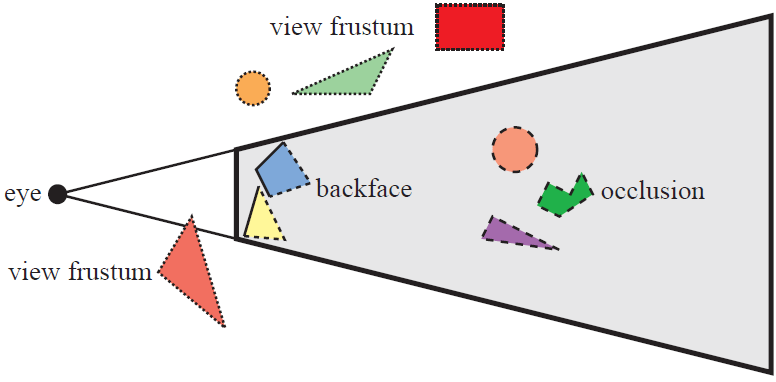
The core motivation for culling is performance. Every command sent to the GPU to draw something (a "draw call") has a CPU cost associated with preparing it. Culling reduces the number of objects the CPU even considers for drawing, freeing it up for other tasks and preventing the GPU from waiting idly.

To understand this better, let's explore the concept of draw calls and viewport culling.

Applying Culling to Our Plotter

As the article explains, the standard way to perform culling is to compare bounding boxes. We need to define two Axis-Aligned Bounding Boxes (AABBs) in our system:

1. The Data's AABB: This is the bounding box that contains our entire dataset in "world space". If we have N data points, their indices run from 0 to N-1. So, the X-dimension of our data's AABB is [0, N-1].
2. The Canvas's AABB: This is the bounding box of the visible plotting area on the screen. This is defined by the plot window's top-left corner (canvas_pos) and its size (canvas_size).

Our goal is to only iterate over the pixels that are part of the intersection of these two bounding boxes. We will not waste time processing pixels on the left of our data's start or on the right of its end.

Implementation: Clipping the Decimation Loop

The implementation is a straightforward modification of the rendering loop you built in the last lesson. We need to calculate the screen-space X coordinates where our data begins and ends, and then clamp our loop's iteration range to the visible canvas area.

Here's the step-by-step logic:

1. Get the canvas horizontal bounds. These are simply the starting X-coordinate of our plot window and the ending X-coordinate (start + width).

   float canvas_min_x = canvas_pos.x;
   float canvas_max_x = canvas_pos.x + canvas_size.x;
   

2. Find the screen-space coordinates for the start and end of our data. We use the worldToScreen function we've already built. The Y-value doesn't matter for this calculation.

   // Assuming 'all_data' is our std::vector of data points
   ImVec2 data_start_world = { 0.0f, 0.0f };
   ImVec2 data_end_world = { static_cast<float>(all_data.size() - 1), 0.0f };
   
   float data_start_screen_x = worldToScreen(data_start_world, pan, zoom, canvas_pos, canvas_size).x;
   float data_end_screen_x = worldToScreen(data_end_world, pan, zoom, canvas_pos, canvas_size).x;
   

3. Calculate the intersection. The starting point for our loop is the maximum of the canvas start and the data start. The ending point is the minimum of the canvas end and the data end.

   float loop_start_x = std::max(canvas_min_x, data_start_screen_x);
   float loop_end_x = std::min(canvas_max_x, data_end_screen_x);
   

4. Update the decimation loop. We replace our old for loop with one that uses these new, clipped bounds.

   // The new, culled loop for the decimated view
   for (float screen_x = loop_start_x; screen_x < loop_end_x; ++screen_x) {
       // ...
       // Your existing logic for converting screen_x to a world_x_range,
       // querying the MinMaxTree, and adding a primitive.
       // This code block remains unchanged.
       // ...
   }
   

And that's it! If the user pans the view far to the left, data_start_screen_x might be 1500, while canvas_max_x is 900. The resulting loop_end_x would be 900, and loop_start_x would be 1500. Since loop_start_x is greater than loop_end_x, the loop will not execute a single time. We have successfully culled all processing.

Culling in the Raw (Zoomed-In) View

The same principle applies when we're zoomed in and rendering individual line segments. In our previous lesson, we calculated a data_idx_start and data_idx_end to loop through. Culling here is even simpler: we just need to clamp these indices to the valid range of our data array, which is [0, all_data.size() - 1].

This prevents the screenToWorld calculation from producing indices that are out of bounds, which could lead to a crash when trying to access all_data[i].

// Inside the 'else' branch for the raw view

// 1. Calculate the visible indices based on screen boundaries
// (This part is from a previous lesson)
size_t visible_idx_start = screenToWorld(...).x;
size_t visible_idx_end = screenToWorld(...).x;

// 2. CULLING STEP: Clamp these indices to the valid data range.
size_t final_idx_start = std::max((size_t)0, visible_idx_start);
size_t final_idx_end = std::min(all_data.size(), visible_idx_end + 2); // +2 for safety for the i+1 access

// 3. Use the clamped indices in the loop
for (size_t i = final_idx_start; i + 1 < final_idx_end; ++i) {
    // ... existing raw rendering logic to draw line from point i to i+1
}

This simple clamping ensures we never attempt to read data that doesn't exist, making our plotter more robust.

Conclusion

You have now implemented a crucial optimization for our LOD plotter. By adding culling logic, you ensure that the application's workload is always proportional to what is actually visible on screen, not the total size of the dataset or the canvas.

Key Takeaways:

• Culling is the practice of discarding non-visible objects to save CPU and GPU time.
• For our 2D plot, we implement culling by finding the intersection of the data's bounding box and the canvas's bounding box in screen space.
• We use std::max and std::min to "clip" the iteration range of our decimation loop, preventing any work on empty portions of the screen.
• This optimization is essential for maintaining a smooth, interactive experience, especially when navigating vast datasets where most of the data is off-screen at any given time.

What's Next?

With this lesson, the core implementation of the high-performance LOD plotter is complete! You have a system that can intelligently decimate and render massive datasets at interactive frame rates.

In the next module, we will begin the final phase of this project: integration. The very next lesson will focus on connecting the data capture pipeline you built in the earlier modules (the per-thread, lock-free ring buffers) to this plotter. We will make the plot live, updating in real-time as new data flows in from the consumer thread. This will bring us one step closer to a complete, functional telemetry engine.