Why Direct Rendering of Millions of Data Points is Inefficient

1. The Visual Problem: Too Much Data, Too Few Pixels

The most intuitive problem is a mismatch of scales. A typical 4K monitor has about 8.3 million pixels. A high-frequency telemetry system can generate millions of data points per second. Trying to render even a few minutes of this data means mapping an enormous dataset onto a comparatively tiny grid of pixels.

This leads to two issues:

1. Overplotting: Multiple data points fall on the same pixel or are so close they become an indistinguishable blob. The final image is saturated and hides the underlying data distribution.
2. Undersampling/Misrepresentation: The order in which points are drawn, their size, or their transparency can create a final image that is factually wrong. You might see patterns that don't exist or miss important outliers completely.

This isn't just theory. Let's watch a segment from a talk by James A. Bednar on the Datashader library, which was built to solve this exact problem.

As you saw, the naive approach doesn't just fail to show all the data; it can actively lie about it. The image below provides a simple, static illustration of this concept. When data density becomes high, individual points lose their meaning.

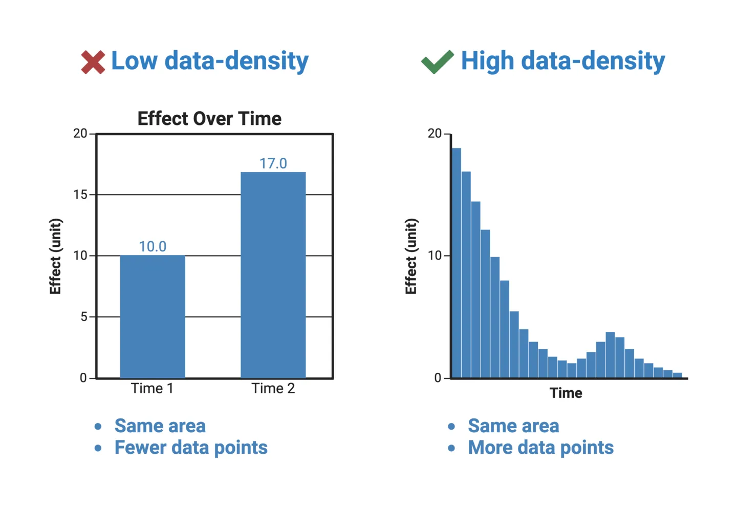
A discussion on Hacker News about ImPlot, a plotting library for ImGui, captures this pixel limitation perfectly.

The key takeaway is that the screen itself is a hard limit. We simply cannot represent every single data point. Therefore, our goal shouldn't be to draw every point, but to represent the underlying data accurately within the available pixels.

2. The Software Pipeline Problem: The Processing Bottleneck

Even if we ignored the visual issues, the software process of rendering is a major source of inefficiency. In our current custom plot, rendering a line chart with N points involves a loop that makes at least N-1 calls to draw_list->AddLine().

Imagine our telemetry engine captures 1 million events. This translates to roughly 1 million draw calls. Each draw call is not free; it involves:

• The CPU calculating vertex positions and colors.
• The CPU pushing this data into a command buffer.
• The CPU instructing the GPU to draw.
• The GPU processing these commands and rasterizing the primitives (drawing pixels).

This creates a classic bottleneck. One part of the system is overwhelmed by the sheer volume of work, slowing everything else down.

This isn't a hypothetical problem. Let's return to the Datashader video, where the speaker demonstrates a popular plotting library, Bokeh, struggling under load. He then introduces a more intelligent pipeline.

The aggregation strategy is the core principle we will adopt for our LOD plotter. By processing the data before we decide what to draw, we can decouple the rendering cost from the data size. We will always send a small, manageable number of draw commands to the GPU, regardless of whether we have a thousand or a billion data points.

3. The Hardware Problem: The Cost of Touching Memory

We've established that millions of draw calls create a bottleneck. But why is the CPU so slow at generating these commands in the first place? The answer lies at the lowest level of your system: memory access and the CPU cache.

Modern CPUs are incredibly fast, but main memory (RAM) is comparatively slow. To bridge this gap, CPUs use small, extremely fast memory banks called caches (L1, L2, L3). When the CPU needs data, it first checks the cache.

• Cache Hit: The data is in the cache. Access is extremely fast.
• Cache Miss: The data is not in the cache. The CPU must stall and wait for the data to be fetched from slow main memory.

Performance in data-intensive applications is often dominated by the cache hit rate. The best way to achieve high cache performance is to access memory sequentially. This is the central idea of Data-Oriented Design (DOD), the philosophy behind our project.

When we iterate through millions of data points to generate draw calls, the layout of that data in memory is paramount. A naive std::vector of complex objects can lead to scattered memory accesses, causing a cascade of cache misses that cripples performance. The CPU spends more time waiting for data than doing actual work.

By organizing our data according to DOD principles—for example, separate, contiguous arrays for timestamps and values—we ensure that when the CPU processes the first data point, the next several hundred are automatically loaded into the cache. This minimizes stalls and maximizes throughput.

Conclusion

Today we've dismantled the problem of rendering large datasets and examined its root causes. A naive approach is inefficient not for one reason, but for three interconnected ones.

Key Takeaways:

• Visual Inefficiency: You have vastly more data points than pixels, leading to overplotting and misleading visualizations. The goal is accurate representation, not direct rendering.
• Software Inefficiency: Issuing a draw call for every data point creates a massive processing bottleneck for the CPU and GPU. The solution is to aggregate data first, then render a fixed-size summary.
• Hardware Inefficiency: Non-sequential memory access patterns cause frequent CPU cache misses, making data processing itself incredibly slow. A data-oriented layout is essential for high throughput.

We now have a deep and precise understanding of the problem we need to solve. Our plotter must not only reduce the number of draw calls but also be built on a data structure that is inherently cache-friendly.

What's Next?

With the "why" firmly established, our next lesson will introduce the "how." We will begin designing the core data structure for our high-performance plotter: the min-max tree. You will learn what this structure is and how it allows us to query vast ranges of data to find the minimum and maximum values in logarithmic time—the first crucial step in building an effective aggregation and decimation algorithm.