Solving Systems with Matrix Operations

1. Understanding the Problem: From Equations to Geometry

A system of linear equations, like the one below, can seem like a simple accounting problem.

2x + y -  z = 8
-3x - y + 2z = -11
-2x + y + 2z = -3

However, by representing it in matrix form as $AX=B$, we unlock a powerful geometric perspective.

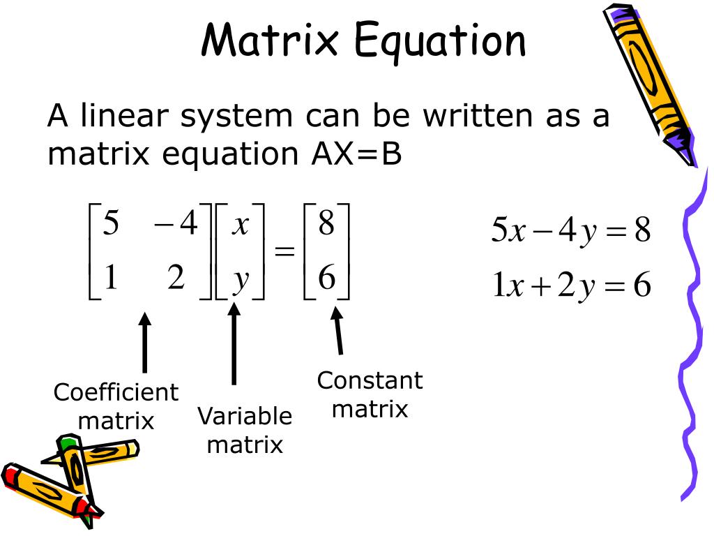
The equation $AX=B$ asks a geometric question: "What vector $X$, when transformed by the matrix $A$, lands on the vector $B$?" Let's build this intuition with a video from 3Blue1Brown.

This geometric viewpoint is incredibly powerful. The question is no longer just about finding numbers that satisfy equations, but about reversing a spatial transformation.

2. The Cleanest Case: Solving with the Matrix Inverse

When the transformation represented by matrix $A$ doesn't collapse space—that is, when $\det (A)\ne 0$—a unique solution exists. In this case, we can reverse the transformation. This reverse transformation is represented by the inverse matrix, denoted $A^{-1}$.

If we have $AX=B$, we can solve for $X$ by applying the inverse transformation to $B$:

where $I$ is the identity matrix.

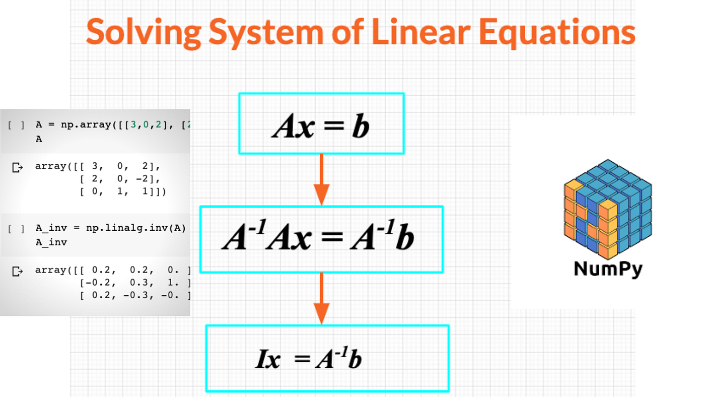
Let's return to the 3Blue1Brown video to see what this "reverse" transformation looks like.

So, if a matrix has an inverse (i.e., its determinant is non-zero), we have a clear path to a unique solution. While computing the inverse manually can be tedious (we'll cover that in the next lesson), in practice, libraries like NumPy have highly optimized functions for this.

The recommended way to solve $AX=B$ in Python is not by finding the inverse and then multiplying, but by using a dedicated solver function, which is more numerically stable and efficient.

import numpy as np




# Let's solve the system from the start of the lesson
A = np.array([[2, 1, -1],
              [-3, -1, 2],
              [-2, 1, 2]])

B = np.array([8, -11, -3])




# We can first check if a unique solution exists
det_A = np.linalg.det(A)
print(f"Determinant of A: {det_A:.1f}") # Output is -1.0, so it's invertible!




# Use the efficient linalg.solve function
X = np.linalg.solve(A, B)

print(f"Solution vector X: {X}") # Output: [ 2.  3. -1.]

This means $x=2$, $y=3$, and $z=-1$ is the unique solution to our system.

3. The Complicated Cases: Zero, One, or Infinite Solutions

What happens if $\det (A)=0$? The transformation collapses space into a lower dimension (e.g., a plane into a line). In this case, there is no inverse transformation—you can't "un-squish" a line back into a plane with a simple function.

This leads to two possibilities for the solution to $AX=B$:

1. No Solution: If the vector $B$ lies outside the collapsed space (the column space of $A$), then no vector $X$ could possibly land on it.
2. Infinitely Many Solutions: If the vector $B$ is within the column space, then not only does at least one solution $X$ exist, but a whole line or plane of vectors (related to the null space of $A$) will also land on $B$.

The following resources delve into these conditions more formally.

To solidify these rules, let's watch a more direct explanation.

To summarize the conditions for solving $AX=B$:

• Unique Solution: If B is in the column space of A AND the null space of A contains only the zero vector (which is true when $\det (A)\ne 0$).
• Infinite Solutions: If B is in the column space of A AND the null space of A is non-trivial (contains more than just the zero vector).
• No Solution: If B is NOT in the column space of A.

This framework is conceptually complete, but how do we implement it algorithmically?

4. The Universal Tool: Gaussian Elimination

Gaussian elimination is a systematic procedure that transforms a system of equations into an "upper triangular" form, which is easy to solve. It works for any square system and, by its result, tells you which of the three cases you're in. The method consists of three stages.

The key is using elementary row operations to simplify the augmented matrix [A|B] into row echelon form, where all elements below the main diagonal are zero. The allowed operations are:

1. Swapping two rows.
2. Multiplying a row by a non-zero constant.
3. Adding a multiple of one row to another row.

These operations change the equations' appearance but not their underlying solution.

Once in row echelon form, the system is trivial to solve from the bottom up. For example, the augmented matrix

corresponds to the equations:

From the last equation, $x_3=3$. You can then substitute this into the second equation to find $x_2$, and so on.

The Solution by Gauss Elimination resource also explains what happens when you have infinite solutions (see Section 3, "Equations which have an infinite number of solutions"). The algorithm reveals this by producing a row of all zeros (e.g., 0 0 0 | 0), indicating a free variable. If it produces a contradiction (e.g., 0 0 0 | 5, which means $0=5$), there is no solution.

Conclusion

In this lesson, we moved from the abstract concept of a determinant to the concrete task of solving systems of linear equations. You now have a comprehensive framework for both understanding and solving the equation $AX=B$.

Key Takeaways:

• Geometric View: Solving $AX=B$ means finding the input vector $X$ that lands on the output vector $B$ after being transformed by $A$.
• The Invertible Case: If $\det (A)\ne 0$, the matrix $A$ is invertible. A unique solution exists and is given by $X=A^{-1}B$.
• The General Conditions: A solution exists if and only if $B$ is in the column space of $A$. If, additionally, $A$ has a non-trivial null space, there are infinitely many solutions.
• Gaussian Elimination: This is the standard algorithm for solving any system of linear equations. It uses row operations to transform the augmented matrix into an easy-to-solve upper triangular form and naturally reveals whether there is a unique solution, no solution, or infinite solutions.

In our next lesson, we will complete the story of the matrix inverse. We've used it conceptually today, and next time we will learn the computational steps for computing the inverse of an invertible matrix, which relies on an extension of the Gaussian elimination process you learned today.