Inverting Matrices

1. The Inverse: Undoing a Transformation

At its core, the inverse of a matrix is an "undo" button. If a matrix $A$ represents a transformation that takes an input vector $x$ to an output vector $b$, its inverse, $A^{-1}$, is the transformation that takes $b$ right back to $x$.

To build a strong intuition for this, let's start with a practical example that frames this concept in a business context.

As the video demonstrates, if applying matrix $P$ gets us from f to m, there must be an inverse matrix $P^{-1}$ that gets us from m back to f. When we combine these two operations, we should end up exactly where we started. This leads to the formal definition of the inverse.

Definition of a Matrix Inverse

For a square matrix $A$, its inverse is a matrix $A^{-1}$ that satisfies the following condition:

where $I$ is the identity matrix—a square matrix with ones on the main diagonal and zeros everywhere else. Applying the identity matrix to any vector leaves the vector unchanged.

2. Conditions for Invertibility

Not all matrices have an inverse. A matrix that has an inverse is called invertible or non-singular. A matrix that does not is called singular. For a matrix to be invertible, it must satisfy two key conditions.

As you just read, the two conditions are:

1. The matrix must be square. It must have the same number of rows and columns ($n\times n$).
2. The determinant of the matrix must be non-zero ($\det (A)\ne 0$).

Let's briefly revisit the intuition for these rules:

• Why square? A linear transformation maps an input space to an output space. An inverse must map that output space back to the original input space. The ritvikmath video's analogy of mapping between "small" and "large" spaces gave a great feel for this. A unique, well-defined inverse generally only exists when the input and output spaces have the same dimension, which corresponds to a square matrix.

• Why non-zero determinant? As we saw in previous lessons, a zero determinant means the transformation squishes space into a lower dimension (e.g., a plane collapses into a line). As 3Blue1Brown explained, you cannot "un-squish" a line back into a plane with a function, because a single input would need to map to multiple outputs. An inverse function can't exist.

3. How to Compute the Inverse

Now for the main event: calculating $A^{-1}$. The method depends on the size of the matrix.

The 2x2 Case: A Simple Formula

For a 2x2 matrix, there is a convenient formula.

For a matrix $A=\left[\begin{array}{cc}a& b\\ c& d\end{array}\right]$, the inverse is:

Example: Let's find the inverse of $A=\left[\begin{array}{cc}4& 7\\ 2& 6\end{array}\right]$.

1. Compute the determinant: $\det (A)=(4)(6)-(7)(2)=24-14=10$.
   Since $\det (A)\ne 0$, the inverse exists.
2. Apply the formula: $$A^{-1}=\frac{1}{10}\left[\begin{array}{cc}6& -7\\ -2& 4\end{array}\right]=\left[\begin{array}{cc}0.6& -0.7\\ -0.2& 0.4\end{array}\right]$$

The n x n Case: Gauss-Jordan Elimination

For matrices larger than 2x2, the formulaic approach becomes unwieldy. The standard algorithm is Gauss-Jordan elimination, which is a direct extension of the Gaussian elimination you learned in the last lesson.

The procedure is as follows:

1. Create an augmented matrix by placing the identity matrix $I$ to the right of your matrix $A$. This looks like $[A|I]$.
2. Use the three elementary row operations (swapping rows, multiplying a row by a non-zero scalar, adding a multiple of one row to another) to transform the left side ($A$) into the identity matrix $I$.
3. As you perform these operations, the right side ($I$) will be transformed into $A^{-1}$. The final form will be $[I|A^{-1}]$.

Let's walk through an example. Find the inverse of $A=\left[\begin{array}{ccc}1& 2& 3\\ 0& 1& 4\\ 0& 0& 1\end{array}\right]$. (This is an upper-triangular matrix, which simplifies the process).

1. Set up the augmented matrix: $$\left[\begin{array}{cccccc}1& 2& 3& 1& 0& 0\\ 0& 1& 4& 0& 1& 0\\ 0& 0& 1& 0& 0& 1\end{array}\right]$$
2. Goal: Transform the left side into $I$. We need to create zeros above the main diagonal. We'll work from bottom to top.
   • Row 3 is already good. We have a 1 in the pivot position.
   • Eliminate the 4 in R2 C3. Use the pivot in R3. Operation: $R_2\leftarrow R_2-4R_3$.
   $$\left[\begin{array}{cccccc}1& 2& 3& 1& 0& 0\\ 0& 1& 0& 0& 1& -4\\ 0& 0& 1& 0& 0& 1\end{array}\right]$$
   • Eliminate the 3 in R1 C3. Operation: $R_1\leftarrow R_1-3R_3$.
   $$\left[\begin{array}{cccccc}1& 2& 0& 1& 0& -3\\ 0& 1& 0& 0& 1& -4\\ 0& 0& 1& 0& 0& 1\end{array}\right]$$
   • Now, eliminate the 2 in R1 C2. Use the pivot in R2. Operation: $R_1\leftarrow R_1-2R_2$.
   $$\left[\begin{array}{cccccc}1& 0& 0& 1& -2& 5\\ 0& 1& 0& 0& 1& -4\\ 0& 0& 1& 0& 0& 1\end{array}\right]$$

The left side is now the identity matrix. The right side is our inverse.

Verification:
An essential final step is to check your work. If you multiply $A$ by your computed $A^{-1}$, you should get the identity matrix.

It works!

The Adjoint Method (A Brief Mention)

Another method you may see in textbooks is the Adjoint method. It involves calculating the determinant, a matrix of cofactors, and the transpose of that matrix (the adjoint).

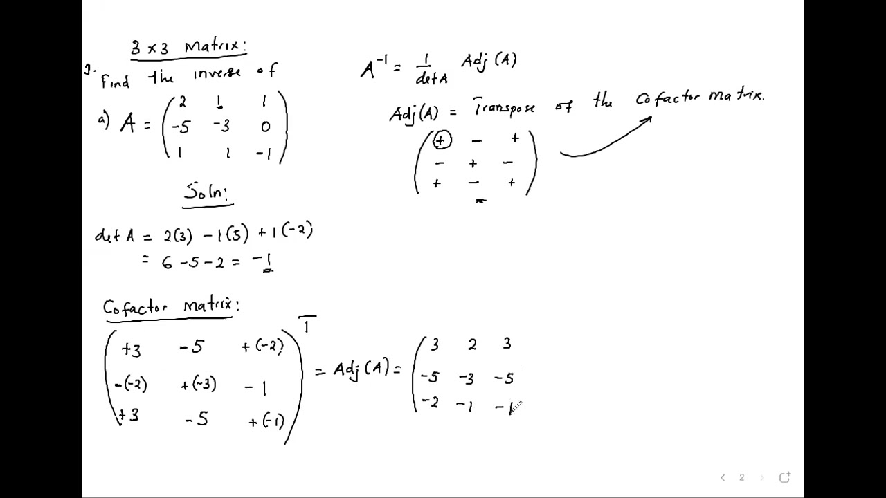
While correct, this method is computationally very expensive for matrices larger than 3x3. For practical purposes, especially in computing and machine learning, Gauss-Jordan elimination is the standard and more efficient technique.

4. Key Properties of Matrix Inverses

Finally, here are a few essential properties of inverses that are useful in algebraic manipulations.

If $A$ and $B$ are invertible matrices of the same size, and $c$ is a non-zero scalar:

• The inverse of the inverse is the original matrix: $(A^{-1}{)}^{-1}=A$
• The inverse of a product is the product of the inverses in reverse order: $(AB{)}^{-1}=B^{-1}{A}^{-1}$
• The inverse of a transpose is the transpose of the inverse: $(A^T{)}^{-1}=(A^{-1}{)}^T$
• The inverse of a matrix scaled by $c$: $(cA{)}^{-1}=\frac{1}{c}{A}^{-1}$

Conclusion

In this lesson, you have closed the loop on matrix inverses. You now understand what they represent, the conditions under which they exist, and how to compute them.

Key Takeaways:

• The inverse matrix $A^{-1}$ reverses the linear transformation performed by matrix $A$, satisfying $A{A}^{-1}=I$.
• A matrix is invertible if and only if it is square and its determinant is non-zero.
• The inverse of a 2x2 matrix can be found with a simple formula.
• For any n x n matrix, Gauss-Jordan elimination is the standard, efficient algorithm for finding the inverse by transforming the augmented matrix $[A|I]$ into $[I|A^{-1}]$.
• Always verify your computed inverse by checking if $A{A}^{-1}=I$.

This lesson marks the end of our first module on Linear Algebra Foundations. You've refreshed your knowledge of vectors, matrices, determinants, and inverses—the essential building blocks. In the next module, we will use these tools to explore matrix decompositions. We'll begin with one of the most important concepts in all of linear algebra: eigenvalues and eigenvectors. These special vectors reveal the intrinsic behavior of a matrix transformation and are the mathematical heart of powerful ML techniques like Principal Component Analysis (PCA).