Multi-Dimensional Aggregation with GROUP BY

The Core Idea: From Raw Data to Aggregated Insights

At its heart, data analysis is often about summarization. You start with thousands or millions of individual records (e.g., sales transactions, user clicks) and need to condense them into a high-level summary (e.g., total sales by region, daily active users). This process is called aggregation.

The GROUP BY clause is the primary tool for aggregation in SQL. It works by taking all the rows that share the same value(s) in a specified column (or columns) and collapsing them into a single row. While doing so, it allows you to perform a calculation across all the original rows in that group using an aggregate function like SUM(), COUNT(), or AVG().

If you've ever used a pivot table in a spreadsheet, you already have an intuitive grasp of what GROUP BY does. They serve the same purpose: to summarize data by one or more categorical dimensions.

Review: Aggregation on a Single Dimension

Let's start with a quick refresher on grouping by a single column. The basic idea is to select a categorical column (a dimension) and an aggregate function applied to a numerical column (a measure). Any column in the SELECT list that is not inside an aggregate function must be in the GROUP BY clause.

The following video provides a concise review of this concept.

Your Turn: A Simple Aggregation

Let's apply this in Metabase. Open a new question using the native SQL editor. We'll answer the business question: "What is our total revenue per product category?"

To do this, you'll need to join the Orders table with the Products table, and then group by the product category.

SELECT
  p.category,
  SUM(o.subtotal) AS total_revenue
FROM orders AS o
JOIN products AS p ON o.product_id = p.id
GROUP BY p.category
ORDER BY total_revenue DESC;

Run this query. You've just transformed thousands of individual orders into a concise summary table, a core task for any analyst.

Grouping by Multiple Dimensions

While grouping by one dimension is useful, real insights often emerge when you slice the data more finely. This is where grouping by multiple columns comes in. Instead of creating groups based on a single column (like category), you create groups based on the unique combination of values from several columns (like category AND region).

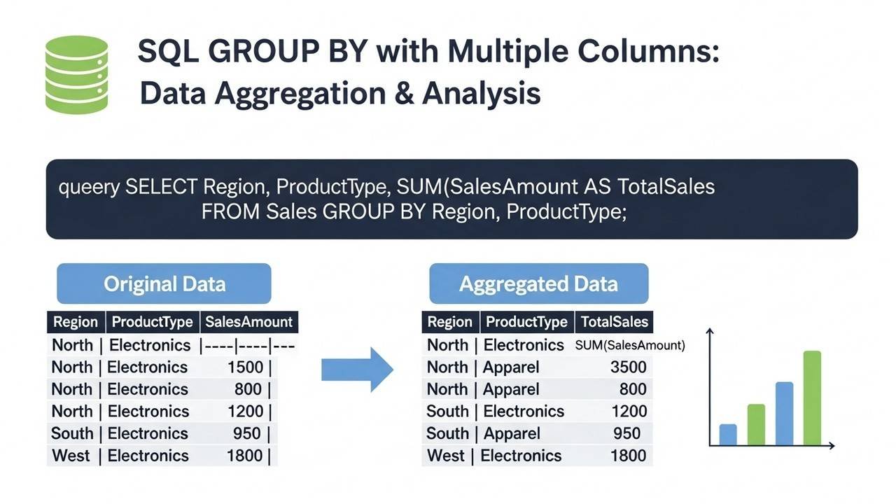
The mechanics are straightforward: you simply add more columns to your GROUP BY clause. The database then treats each unique combination of those columns' values as a single group for aggregation.

Your Turn: Multi-Dimensional Aggregation

Let's make our previous query more granular. Let's answer: "What is our monthly revenue per product category?" This requires grouping by both the category and the month of the order.

To get the month, we can use a date function. In PostgreSQL (the database behind Metabase's sample data), DATE_TRUNC('month', timestamp_column) is perfect for this. It truncates a date/time value down to the beginning of the specified period (in this case, the month).

Modify your previous query to look like this:

SELECT
  p.category,
  DATE_TRUNC('month', o.created_at)::date AS order_month,
  SUM(o.subtotal) AS total_revenue
FROM orders AS o
JOIN products AS p ON o.product_id = p.id
GROUP BY
  p.category,
  order_month
ORDER BY
  p.category,
  order_month;

(Note: ::date is a PostgreSQL-specific shortcut to cast the timestamp to a simple date, which makes the output cleaner.)

When you run this, you'll see a much more detailed breakdown. You're no longer just seeing total revenue for "Gizmo"; you're seeing revenue for "Gizmo" in January, "Gizmo" in February, and so on. This multi-dimensional view is essential for trend analysis.

Filtering: WHERE vs. HAVING

Once you start grouping, you'll inevitably want to filter the results. SQL provides two clauses for filtering, WHERE and HAVING, and their distinction is crucial in analytical queries.

1. WHERE filters rows before aggregation. It acts on the raw data in your tables.
2. HAVING filters groups after aggregation. It acts on the summarized rows created by GROUP BY and can use aggregate functions in its conditions.

Think of it as a two-step filtering process: WHERE cleans the raw data first, then GROUP BY and the aggregate functions run, and finally HAVING cleans the resulting summary rows.

This video offers an excellent explanation of the difference.

Your Turn: Filtering Your Aggregates

Let's refine our previous query with both WHERE and HAVING. Imagine this business request: "For our 'Gadget' category, which months had revenue over $1,500?"

• "For our 'Gadget' category" is a filter on the raw data -> Use WHERE.
• "which months had revenue over $1,500" is a filter on the aggregated result -> Use HAVING.

Modify your query to include these clauses:

SELECT
  p.category,
  DATE_TRUNC('month', o.created_at)::date AS order_month,
  SUM(o.subtotal) AS total_revenue
FROM orders AS o
JOIN products AS p ON o.product_id = p.id
WHERE p.category = 'Gadget' -- Filter rows before grouping
GROUP BY
  p.category,
  order_month
HAVING SUM(o.subtotal) > 1500 -- Filter groups after aggregation
ORDER BY
  order_month;

Running this query gives you a precise answer to a complex business question by using the full power of the SELECT...FROM...WHERE...GROUP BY...HAVING...ORDER BY sequence. Understanding this sequence is a major step toward thinking like a data analyst.

Conclusion

In this lesson, you moved from simple queries to a core analytical SQL pattern: multi-dimensional aggregation. You've seen how GROUP BY is used to summarize vast amounts of data and how to slice that data across multiple dimensions to get granular insights. Critically, you've also learned the difference between WHERE and HAVING for pre- and post-aggregation filtering.

Key Takeaways:

• Aggregation is the process of summarizing raw data into meaningful metrics using functions like SUM(), COUNT(), and AVG().
• GROUP BY collapses rows based on the unique values in one or more columns (dimensions) to perform these aggregations.
• Grouping by multiple columns creates more granular summary groups based on the unique combinations of those columns.
• The WHERE clause filters individual rows before they are grouped and aggregated.
• The HAVING clause filters the final groups after aggregation, based on the value of the aggregate function.

In our next lesson, we will build on this by learning how to create our own custom categories for grouping. What if you wanted to group products into 'High Price' and 'Low Price' buckets before aggregating? You'll learn how to do just that using CASE statements, giving you even more flexibility in your analysis.