Solving Kinematic Problems with Variable Acceleration

1. Beyond Constant Acceleration

In your foundational mechanics studies, you worked extensively with the equations of uniform acceleration (often called the "suvat" equations):

• $v=v_0+at$
• $x=x_0+v_{0}t+\frac{1}{2}a{t}^2$
• $v^2=v_0^2+2a(x-x_0)$

These are powerful, but only when $a$ is a constant. When acceleration varies, these algebraic shortcuts are no longer valid. We must return to the fundamental definitions of velocity and acceleration, which are inherently based on calculus:

By using these definitions, we can handle any situation where acceleration is a known function. We will systematically explore the three primary scenarios you will encounter:

1. Acceleration is a function of time, $a(t)$.
2. Acceleration is a function of velocity, $a(v)$.
3. Acceleration is a function of position, $a(x)$.

The following chart provides a great visual summary of 1-D kinematics. Note the clear distinction between the "Constant Acceleration" section (3a), which leads to the familiar algebraic equations, and the "Variable Acceleration" section (3c), which relies on integration, our focus for today.

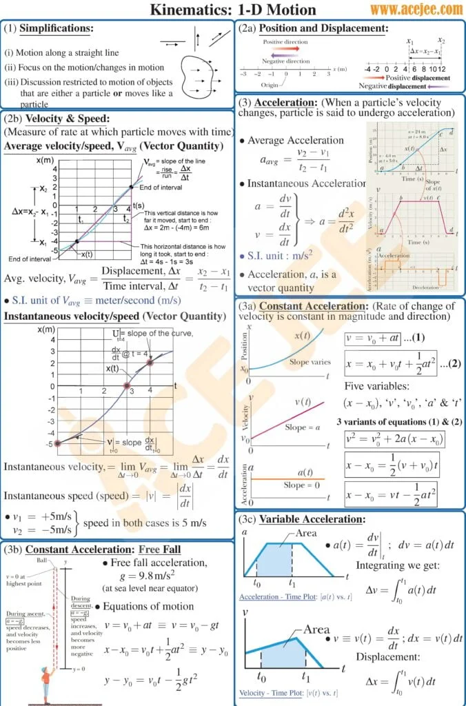
2. Case 1: Acceleration as a Function of Time, $a(t)$

This is the most direct extension of constant acceleration. If we know how acceleration changes with time, we can find velocity and then position by performing successive integrations.

Starting from $a(t)=\frac{dv}{dt}$, we can find the change in velocity from an initial time $t_0$ (often 0) to a later time $t$ by integrating:

Once we have the velocity function $v(t)$, we can repeat the process to find the position function $x(t)$, starting from $v(t)=\frac{dx}{dt}$:

The key steps are direct integration and using the initial conditions ($x_0,v_0$) to solve for the constants of integration.

The following video walks through a clear example of this process.

For a concise text-based explanation, you can refer to the resource below.

3. Case 2: Acceleration as a Function of Velocity, $a(v)$

This scenario is very common in realistic mechanics problems, especially those involving resistive forces like air drag or friction that depend on speed. Here, $a$ is a function of $v$, so we cannot directly integrate with respect to time.

We start with $a(v)=\frac{dv}{dt}$. The key technique here is separation of variables. We algebraically rearrange the equation to gather all terms involving $v$ on one side and all terms involving $t$ on the other:

Now we can integrate both sides over the corresponding intervals:

This gives us a relationship between time and velocity, often in the form $t(v)$. We may then need to algebraically solve for $v$ to get the explicit function $v(t)$.

This method is essential for problems like Irodov 1.23, which asks for the distance and time taken for an object to stop when its deceleration is given as $w=a\sqrt{v}$. You now have the fundamental tool to approach such a problem.

4. Case 3: Acceleration as a Function of Position, $a(x)$

This case arises in systems where the force depends on location, such as a mass on a spring ($F=-kx$) or gravitational force over large distances ($F=-GMm/x^2$). It requires a clever manipulation using the chain rule.

Starting with $a=\frac{dv}{dt}$, we can't integrate with respect to time because $a$ is given as a function of $x$, not $t$. We need a way to relate $dv$ to $dx$. We achieve this using the chain rule:

Since $\frac{dx}{dt}=v$, we arrive at a new, extremely useful expression for acceleration:

Rearranging this gives us a relationship that is now separable in terms of $v$ and $x$:

This is a powerful result. As you might recognize from your mechanics background, it is effectively a statement of the work-energy theorem. Integrating both sides, $\int Fdx=\int (ma)dx$ on the left (Work) and $\int (mv)dv=\Delta (\frac{1}{2}m{v}^2)$ on the right (Change in Kinetic Energy).

Integrating our kinematic expression gives velocity as a function of position:

The following video provides an excellent and concise explanation of this derivation.

Once you have $v(x)$, if you need to find the position as a function of time, $x(t)$, you can proceed with a second integration step using separation of variables on $v(x)=\frac{dx}{dt}$.

Problems like Irodov 1.22, where velocity is given as $v=\alpha \sqrt{x}$, are a direct application of this method. By differentiating this expression with respect to time, you can find the acceleration and analyze the motion.

Conclusion

In this lesson, you've moved beyond the limitations of constant acceleration kinematics. You have learned the three primary scenarios for variable acceleration in one dimension and the specific calculus-based strategy required for each.

Your key takeaways are:

• For constant acceleration, use algebraic kinematic equations. For variable acceleration, you must use integration.
• The strategy depends on the functional form of the acceleration:
  • If $a=a(t)$: Integrate twice with respect to time. $v(t)=\int a(t)dt$ and $x(t)=\int v(t)dt$.
  • If $a=a(v)$: Use separation of variables on $a=dv/dt$ to get $\int \frac{dv}{a(v)}=\int dt$.
  • If $a=a(x)$: Use the chain rule identity $a=v\frac{dv}{dx}$ and integrate the separated form $\int a(x)dx=\int vdv$.

You are now equipped with the core techniques to solve a much broader and more realistic class of dynamics problems. This skill is not just an isolated topic but a recurring theme in advanced mechanics.

In the next lesson, we will continue to apply our calculus tools by exploring forces. Specifically, you will learn to calculate the work done by non-conservative and path-dependent vector force fields using the line integrals you studied in the first module. This will connect the forces that cause these variable accelerations to the concepts of work and energy.