MLE as Loss Function Minimization

Welcome to the first lesson of our module on estimation and inference. In the previous module, we developed a solid understanding of probability distributions, culminating in the tools to dissect and manipulate the multivariate Gaussian. We saw how to model the joint behavior of random variables and how to derive their marginal and conditional distributions.

The natural next question is: given a family of probability models (like Gaussians), and a set of real-world data, how do we choose the specific model that best explains the data? This is the problem of parameter estimation. In this lesson, we will explore one of the most fundamental and powerful frameworks for this: Maximum Likelihood Estimation (MLE). Our goal is to formulate the MLE principle and, crucially, connect it to the loss functions you routinely minimize when training deep learning models, such as Mean Squared Error and cross-entropy.

1. The Principle of Maximum Likelihood

Imagine you have a collection of data points, and you hypothesize they were generated from some parametric probability distribution, say a Gaussian. A Gaussian is defined by its mean $\vmu$ and covariance $\mSigma$ . Which values of $\vmu$ and $\mSigma$ are the "best" fit for your data?

Maximum Likelihood Estimation provides a beautifully simple answer: choose the parameters that make your observed data the most probable.

Let your dataset be $X = {x_{1}, \dots, x_{N}}$ and your model's parameters be $\vtheta$ . The probability (or probability density) of observing the data given the parameters is $p (X ∣ \vtheta)$ . This function, when viewed as a function of $\vtheta$ for a fixed $X$ , is called the likelihood function, often denoted $L (\vtheta ∣ X)$ . The MLE principle states that the best estimate for $\vtheta$ is the one that maximizes this function:

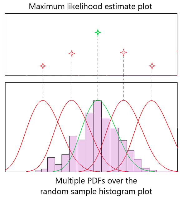
\vtheta^_{MLE} = ar g \vtheta max L (\vtheta ∣ X) = ar g \vtheta max p (X ∣ \vtheta)

The image below provides a great intuition for this. The histogram shows an empirical distribution of data. The red curves are different candidate probability density functions (PDFs), each corresponding to a different choice of parameters. The green curve is the one whose parameters place the highest probability mass on the observed data points, making it the maximum likelihood estimate.

This plot illustrates the core idea of MLE. Among several possible probability distributions (the curves), the one that assigns the highest joint probability to the observed data samples (the histogram) is selected. The peak of this "best fit" distribution (the green star) corresponds to the maximum likelihood estimate.

To formalize this and see it in action, let's turn to a foundational text.

22.7. Maximum Likelihood

This chapter from "Dive into Deep Learning" provides a clear introduction to the MLE principle. It starts with a brief Bayesian justification and then works through a concrete example.

Please read the first section, The Maximum Likelihood Principle, up to and including the subsection "A Concrete Example". Pay close attention to the coin-flipping scenario. The derivation shows how to analytically find the parameter \theta (the probability of heads) that maximizes the likelihood of observing a specific sequence of flips. This is a canonical example of MLE for a discrete distribution (the Bernoulli distribution).

As the text shows, for a sequence of coin flips with $n_{H}$ heads and $n_{T}$ tails, the likelihood is $L (θ) = θ^{n_{H}} (1 - θ)^{n_{T}}$ . By taking the derivative with respect to $θ$ and setting it to zero, we find the intuitive result $θ^_{M L E} = \frac{n _{H}}{n _{H} + n _{T}}$ .

2. The Negative Log-Likelihood: From Probability to Loss

While maximizing the likelihood function $L (\vtheta ∣ X)$ is correct in principle, it's often impractical. If our data points are independent and identically distributed (i.i.d.), the total likelihood is the product of individual probabilities:

L (\vtheta ∣ X) = p (X ∣ \vtheta) = i = 1 \prod N p (x_{i} ∣ \vtheta)

Multiplying a large number of probabilities (which are less than 1) can quickly lead to numerical underflow in a computer. Furthermore, taking derivatives of a long product is cumbersome. The solution is to work with the log-likelihood instead. Since the logarithm is a strictly monotonically increasing function, maximizing the likelihood is equivalent to maximizing the log-likelihood:

\vtheta^_{MLE} = ar g \vtheta max lo g L (\vtheta ∣ X) = ar g \vtheta max i = 1 \sum N lo g p (x_{i} ∣ \vtheta)

This formulation handily converts products into sums, which are numerically stable and much easier to differentiate.

In deep learning, we are accustomed to minimizing a loss function. We can frame our MLE problem as a minimization by simply taking the negative log-likelihood (NLL):

\vtheta^_{MLE} = ar g \vtheta min [- i = 1 \sum N lo g p (x_{i} ∣ \vtheta)]

This expression, $- lo g p (X ∣ \vtheta)$ , is the fundamental bridge connecting probabilistic modeling to the loss functions you use every day.

22.7. Maximum Likelihood

The same article provides an excellent justification for using the negative log-likelihood.

Please read the sections Numerical Optimization and the Negative Log-Likelihood and Maximum Likelihood for Continuous Variables. The text outlines three key reasons for this shift: Numerical stability: avoiding underflow by summing logs instead of multiplying probabilities. Simpler gradients: derivatives of sums are simpler than derivatives of products. Information-theoretic connection: the average NLL is equivalent to cross-entropy. The second section you'll read justifies extending this entire framework to continuous variables by replacing probabilities with probability densities.

3. MLE as the Foundation for Common Loss Functions

Now we'll make the connection explicit for two of the most important loss functions in machine learning.

Mean Squared Error (MSE) for Regression

In regression problems, we often use MSE loss without a second thought. But why is squaring the error the "right" thing to do? MLE provides the answer.

The standard assumption in linear regression is that the target variable $y_{i}$ is generated from a linear function of the features $x_{i}$ plus some random noise $ϵ_{i}$ .

y_{i} = f (x_{i}; \vtheta) + ϵ_{i}

where $f (x_{i}; \vtheta)$ is our model's prediction (e.g., $\vtheta^{T} x_{i}$ ). The crucial step is assuming the noise is independent and identically distributed according to a Gaussian distribution with zero mean and variance $σ^{2}$ , i.e., $ϵ_{i} \sim N (0, σ^{2})$ .

This implies that the conditional probability of observing $y_{i}$ is also Gaussian, with its mean centered on our model's prediction:

p (y_{i} ∣ x_{i}; \vtheta, σ) = N (y_{i} ∣ f (x_{i}; \vtheta), σ^{2})

The following video provides a concise derivation showing how minimizing the NLL of this model leads directly to the least squares objective.

Least Squares vs Maximum Likelihood

This video by DataMListic clearly connects the least squares method to maximum likelihood estimation under a Gaussian assumption.

Watch the quick recap of linear regression. Then, follow the core derivation from the connection. This part shows step-by-step how maximizing the log-likelihood of the data under the Gaussian noise model is equivalent to minimizing the sum of squared errors. Finally, the conclusion at the end discusses the powerful implication: this probabilistic viewpoint allows us to generalize regression by assuming different noise distributions, leading to Generalized Linear Models.

Let's recap the key mathematical steps. The negative log-likelihood for the entire dataset is:

NLL (\vtheta, σ) = - i = 1 \sum N lo g (\frac{1}{2 π σ ^{2}} exp (- \frac{( y _{i} - f ( x _{i} ; \vtheta ) ) ^{2}}{2 σ ^{2}}))

Using log rules, this simplifies to:

NLL (\vtheta, σ) = i = 1 \sum N (lo g (2 π σ^{2}) + \frac{( y _{i} - f ( x _{i} ; \vtheta ) ) ^{2}}{2 σ ^{2}})

= \frac{N}{2} lo g (2 π σ^{2}) + \frac{1}{2 σ ^{2}} i = 1 \sum N (y_{i} - f (x_{i}; \vtheta))^{2}

To find the optimal parameters $\vtheta$ that minimize this NLL, we can ignore terms that don't depend on $\vtheta$ . The first term is constant with respect to $\vtheta$ , and so is the $1/ (2 σ^{2})$ factor. Thus, minimizing the NLL is perfectly equivalent to minimizing:

i = 1 \sum N (y_{i} - f (x_{i}; \vtheta))^{2}

This is exactly the Sum of Squared Errors (SSE) objective. Minimizing MSE is therefore equivalent to performing Maximum Likelihood Estimation under the assumption of additive Gaussian noise.

Cross-Entropy for Classification

A similar story unfolds for classification. Here, our model outputs a probability distribution over $C$ classes. For a single data point $x_{i}$ , the model predicts a vector of probabilities $p_{i} = (p_{i 1}, \dots, p_{i C})$ , where $p_{i c}$ is the probability that $x_{i}$ belongs to class $c$ . The true label can be represented as a one-hot vector $y_{i}$ , where $y_{i c} = 1$ if the true class is $c$ , and 0 otherwise.

The underlying probability distribution for a single trial with multiple outcomes is the Categorical distribution. The probability of observing the outcome $y_{i}$ given the model's predictions $p_{i}$ is:

p (y_{i} ∣ p_{i}) = c = 1 \prod C p_{i c}^{y_{i c}}

This elegant expression simply picks out the predicted probability for the correct class, since all other terms in the product have an exponent of 0.

Now, let's find the negative log-likelihood for a dataset of $N$ points:

NLL (\vtheta) = - i = 1 \sum N lo g (c = 1 \prod C p_{i c}^{y_{i c}}) = - i = 1 \sum N c = 1 \sum C y_{i c} lo g (p_{i c})

This expression is precisely the cross-entropy loss used ubiquitously in deep learning for classification tasks. Therefore, minimizing cross-entropy loss is equivalent to performing Maximum Likelihood Estimation assuming the data is generated from a Categorical distribution.

The plot below compares the shape of the MSE and cross-entropy (labeled "Entropy Loss") for a binary classification problem where the true label is 1.

This plot shows the loss for a single data point with a true label of 1, as a function of the model's predicted probability for that label. Cross-entropy (Entropy Loss) penalizes confident incorrect predictions (prediction close to 0) far more heavily than MSE. The gradient of the cross-entropy loss is much steeper for poor predictions, which typically leads to faster training.

Conclusion

In this lesson, we have demystified the origin of two of the most common loss functions in machine learning by grounding them in the principle of Maximum Likelihood Estimation. This provides a coherent probabilistic foundation for what might otherwise seem like arbitrary choices.

Key Takeaways:

Maximum Likelihood Estimation (MLE) is a principle for fitting a probabilistic model by finding the parameters that maximize the likelihood of the observed data.
In practice, we minimize the Negative Log-Likelihood (NLL) for reasons of numerical stability and analytical convenience.
Minimizing Mean Squared Error (MSE) loss in a regression setting is equivalent to performing MLE on a model that assumes the data contains additive i.i.d. Gaussian noise.
Minimizing Cross-Entropy loss in a classification setting is equivalent to performing MLE on a model that assumes the data is generated from a Bernoulli or Categorical distribution.

We have focused on finding the single best "point estimate" for our model parameters. However, this approach doesn't allow us to incorporate any prior beliefs we might have about the parameters. In our next lesson, we will introduce a Bayesian perspective with Maximum a Posteriori (MAP) estimation, which will reveal an equally profound connection between probabilistic priors and regularization techniques like L1 and L2.