Multivariate Gaussian Conditioning with Schur Complements

1. Partitioning a Gaussian Vector

Let's consider a $D$-dimensional random vector $\mathbf{x}$ that follows a multivariate Gaussian distribution, $\mathbf{x}\sim \mathcal{N}(\text{vmu},\text{mSigma})$. Suppose we partition this vector into two components, ${\mathbf{x}}_a$ of dimension $N$ and ${\mathbf{x}}_b$ of dimension $M$, where $N+M=D$.

This partitioning induces a corresponding block structure in the mean vector $\text{vmu}$ and the covariance matrix $\text{mSigma}$:

Here, ${\text{mSigma}}_{aa}$ is the $N\times N$ covariance matrix of ${\mathbf{x}}_a$, ${\text{mSigma}}_{bb}$ is the $M\times M$ covariance matrix of ${\mathbf{x}}_b$, and ${\text{mSigma}}_{ab}$ (which is the transpose of ${\text{mSigma}}_{ba}$) is the $N\times M$ cross-covariance matrix between ${\mathbf{x}}_a$ and ${\mathbf{x}}_b$.

Our goal is to find the distributions $p({\mathbf{x}}_a)$ (the marginal) and $p({\mathbf{x}}_a|{\mathbf{x}}_b)$ (the conditional).

2. Marginal Distributions: The Simple Case

The marginal distribution $p({\mathbf{x}}_a)$ is what we get when we "ignore" or integrate out ${\mathbf{x}}_b$: $p({\mathbf{x}}_a)=\int p({\mathbf{x}}_a,{\mathbf{x}}_b)d{\mathbf{x}}_b$. Intuitively, if you project the ellipsoidal cloud of points from the joint distribution onto the subspace of ${\mathbf{x}}_a$, you get the marginal distribution.

One of the remarkable properties of the Gaussian is that this marginal is also Gaussian. The proof is surprisingly elegant and relies on the affine transformation property we studied last time. The following video provides a clear explanation.

As the video proves, the result is beautifully simple. The marginal distribution of ${\mathbf{x}}_a$ is obtained by simply selecting the corresponding blocks from the mean vector and covariance matrix:

3. Conditional Distributions: Slicing the Gaussian

Finding the conditional distribution $p({\mathbf{x}}_a|{\mathbf{x}}_b)$ is more involved but arguably more important for inference. It answers the question: "Given that I've observed the value of ${\mathbf{x}}_b$, what is my updated belief about the distribution of ${\mathbf{x}}_a$?" Geometrically, this is like taking a "slice" through the joint probability density at a fixed value of ${\mathbf{x}}_b$.

The resulting distribution is, once again, a Gaussian. The video below provides the intuition and the formulas.

The conditional distribution $p({\mathbf{x}}_a|{\mathbf{x}}_b)$ is given by $\mathcal{N}({\mathbf{x}}_a|{\text{vmu}}_{a|b},{\text{mSigma}}_{a|b})$, where:

• Conditional Mean: ${\text{vmu}}_{a|b}={\text{vmu}}_a+{\text{mSigma}}_{ab}{\text{mSigma}}_{bb}^{-1}({\mathbf{x}}_b-{\text{vmu}}_b)$
• Conditional Covariance: ${\text{mSigma}}_{a|b}={\text{mSigma}}_{aa}-{\text{mSigma}}_{ab}{\text{mSigma}}_{bb}^{-1}{\text{mSigma}}_{ba}$

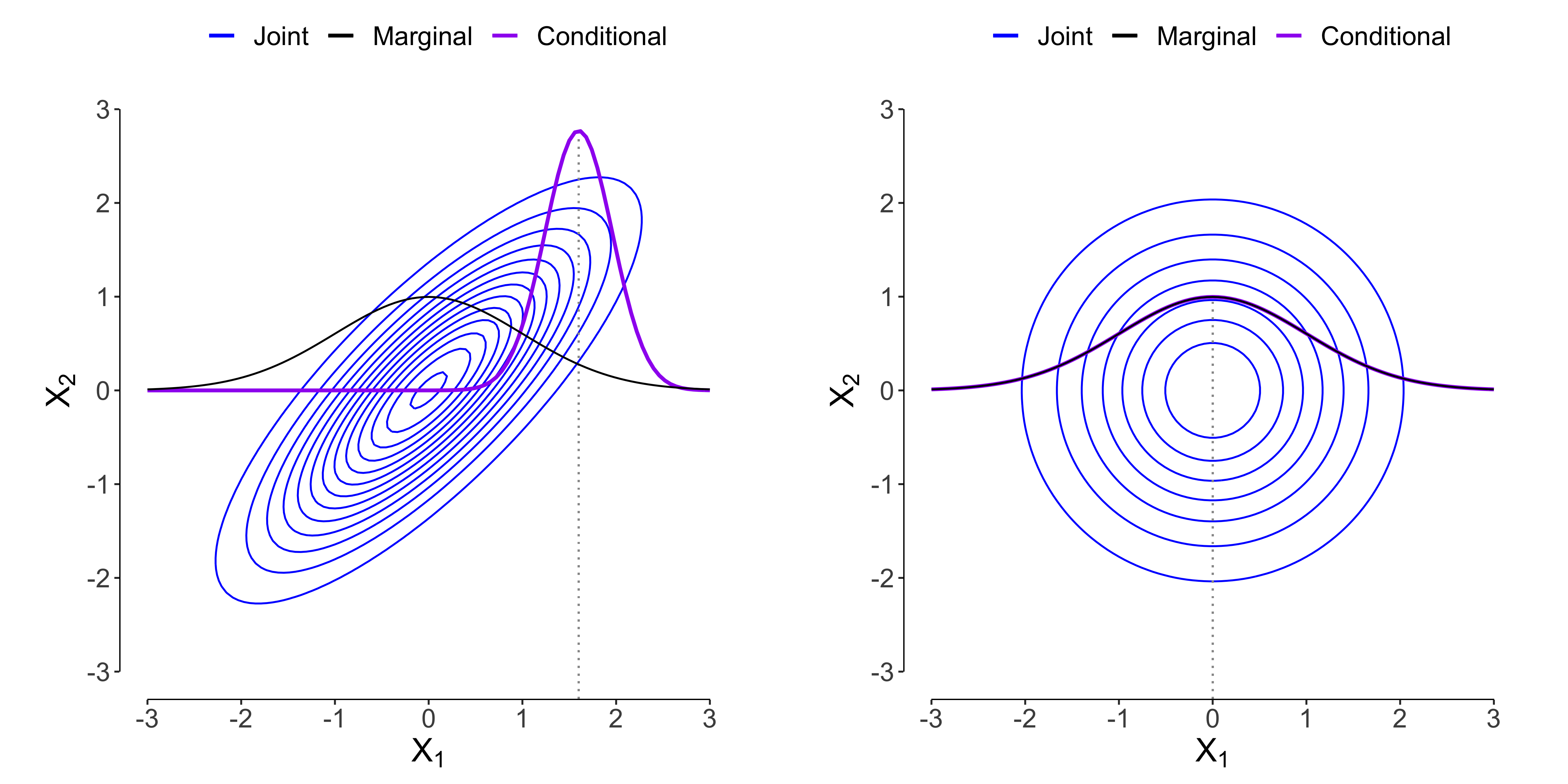
The conditional mean is a linear function of the observed value ${\mathbf{x}}_b$. It starts at the prior mean ${\text{vmu}}_a$ and adjusts it based on how far the observed ${\mathbf{x}}_b$ is from its own mean ${\text{vmu}}_b$, scaled by the correlation term ${\text{mSigma}}_{ab}{\text{mSigma}}_{bb}^{-1}$.

The conditional covariance, interestingly, does not depend on the value of ${\mathbf{x}}_b$. Observing ${\mathbf{x}}_b$ reduces our uncertainty about ${\mathbf{x}}_a$, and the amount of this reduction is fixed. The term ${\text{mSigma}}_{ab}{\text{mSigma}}_{bb}^{-1}{\text{mSigma}}_{ba}$ is always positive semi-definite, so the conditional covariance ${\text{mSigma}}_{a|b}$ is always "smaller" than or equal to the marginal covariance ${\text{mSigma}}_{aa}$.

The image below nicely illustrates these concepts for a 2D Gaussian.

4. Derivation using the Schur Complement

Now, where do these formulas come from? The derivation is a beautiful piece of matrix algebra that hinges on understanding the structure of the inverse of a partitioned matrix. The key component that emerges is the Schur complement.

The article "The Venerable Gaussian" provides an excellent, self-contained derivation. We'll walk through it in two steps. First, we'll master the necessary matrix machinery.

With the Schur complement and the block matrix inverse formulas in hand, we can now tackle the main derivation. The strategy is to write out the quadratic form in the exponent of the joint distribution $p({\mathbf{x}}_a,{\mathbf{x}}_b)$ and algebraically manipulate it to separate it into two parts: one corresponding to $p({\mathbf{x}}_b)$ and another corresponding to $p({\mathbf{x}}_a|{\mathbf{x}}_b)$. By comparing the latter part to the standard Gaussian form, we can "read off" the parameters of the conditional distribution.

This derivation is a cornerstone of many proofs in machine learning. It shows how conditioning on a Gaussian variable involves a linear update to the mean and a reduction in covariance given by the Schur complement.

Conclusion

In this lesson, we have explored the fundamental properties of marginal and conditional distributions within a multivariate Gaussian framework. These operations are essential tools for probabilistic inference.

Key Takeaways:

• Partitioning: A multivariate Gaussian vector can be partitioned into sub-vectors, with corresponding blocks in the mean vector and covariance matrix.
• Marginalization: The marginal distribution of a subset of variables is also Gaussian. Its parameters are found by simply taking the corresponding blocks of the original mean and covariance matrix. This is equivalent to projecting the distribution onto a subspace.
• Conditioning: The conditional distribution of one subset of variables given another is also Gaussian. This is equivalent to taking a slice through the joint density.
• Schur Complement: The covariance matrix of the conditional distribution is given by the Schur complement of the appropriate block in the joint covariance matrix. This reflects the reduction in uncertainty from observing a correlated variable.

We now have the tools to manipulate and reason about joint Gaussian distributions. In our next lesson, we will shift our focus from the properties of distributions to the problem of estimation. We will explore Maximum Likelihood Estimation (MLE) and see how minimizing common loss functions like Mean Squared Error is equivalent to finding the MLE for a Gaussian model of the data.