MAP Estimation and Regularization Priors

In our previous lesson, we established Maximum Likelihood Estimation (MLE) as a powerful principle for fitting models, demonstrating its direct connection to the loss functions you regularly use, like MSE and cross-entropy. MLE seeks the parameters $\vtheta$ that make the observed data $X$ most probable, by maximizing the likelihood $p (X ∣ \vtheta)$ . While fundamental, this approach has a significant limitation: it can be prone to overfitting. MLE will happily choose extreme parameter values if they perfectly fit the training data, without regard for whether those values are "reasonable" or will generalize well.

Today, we move from this frequentist perspective to a Bayesian one by introducing Maximum a Posteriori (MAP) estimation. Instead of just maximizing the data's likelihood, MAP incorporates prior beliefs about what constitutes a "good" set of parameters. This will allow us to find the most probable parameters given the data. As you'll see, this small but profound shift provides a principled, probabilistic justification for the L1 and L2 regularization techniques that are indispensable for training modern deep learning models.

1. From Likelihood to Posterior Probability

The core of Bayesian reasoning is Bayes' theorem. When applied to parameter estimation, it allows us to update our beliefs about the parameters $\vtheta$ after observing data $X$ . The theorem states:

p (\vtheta ∣ X) = \frac{p ( X ∣ \vtheta ) p ( \vtheta )}{p ( X )}

Let's break down these terms in the context of our goal:

Posterior, $p (\vtheta ∣ X)$ : The probability of the parameters after seeing the data. This is what we want to maximize.
Likelihood, $p (X ∣ \vtheta)$ : The probability of the data given the parameters. This is the same term we maximized in MLE.
Prior, $p (\vtheta)$ : The probability of the parameters before seeing any data. This is the crucial new ingredient, encoding our prior beliefs. For example, we might believe that smaller parameter values are more likely than very large ones.
Evidence, $p (X)$ : The marginal probability of the data. Since we are maximizing with respect to $\vtheta$ , and $p (X)$ does not depend on $\vtheta$ , we can treat it as a normalizing constant and ignore it for the optimization.

Therefore, MAP estimation seeks the parameters that maximize the posterior probability:

\vtheta^_{MAP} = ar g \vtheta max p (\vtheta ∣ X) \propto ar g \vtheta max p (X ∣ \vtheta) p (\vtheta)

As we did with MLE, we can work with the log of this expression to make it more tractable. Maximizing the posterior is equivalent to maximizing the log-posterior:

\vtheta^_{MAP} = ar g \vtheta max [lo g p (X ∣ \vtheta) + lo g p (\vtheta)]

Flipping this into a minimization problem gives us a formulation that should look very familiar:

\vtheta^_{MAP} = ar g \vtheta min [- lo g p (X ∣ \vtheta) - lo g p (\vtheta)]

Compare this to the Negative Log-Likelihood (NLL) objective from MLE: $ar g min_{\vtheta} [- lo g p (X ∣ \vtheta)]$ . The MAP objective is simply the NLL (our familiar loss function) plus a new term, $- lo g p (\vtheta)$ . This new term acts as a regularizer, penalizing parameter values that are unlikely according to our prior belief.

2. Gaussian Priors and L2 Regularization

Let's make this concrete. What happens if we choose a specific, common prior for our parameters? A very natural belief is that model parameters should be small and centered around zero. This helps prevent individual parameters from having an outsized influence, a hallmark of overfitting. The Gaussian distribution is a perfect way to mathematically express this belief.

Let's assume a zero-mean Gaussian prior for each parameter $θ_{j}$ , with some variance $τ^{2}$ . This means we believe $θ_{j} \sim N (0, τ^{2})$ . The prior for the entire parameter vector $\vtheta$ is:

p (\vtheta) = j \prod \frac{1}{2 π τ ^{2}} exp (- \frac{θ _{j}^{2}}{2 τ ^{2}})

Now, let's derive the regularization term, $- lo g p (\vtheta)$ :

- lo g p (\vtheta) = - j \sum lo g (\frac{1}{2 π τ ^{2}} exp (- \frac{θ _{j}^{2}}{2 τ ^{2}}))

= - j \sum (- lo g (2 π τ^{2}) - \frac{θ _{j}^{2}}{2 τ ^{2}})

= N lo g (2 π τ^{2}) + \frac{1}{2 τ ^{2}} j \sum θ_{j}^{2}

The first term is a constant with respect to $\vtheta$ , so we can drop it from the minimization. The second term is $\frac{1}{2 τ ^{2}} ∣∣ \vtheta ∣ ∣_{2}^{2}$ .

Let's combine this with our NLL from the previous lesson for a regression problem, where $- lo g p (X ∣ \vtheta)$ was proportional to the sum of squared errors, $\frac{1}{2 σ ^{2}} \sum_{i} (y_{i} - f (x_{i}; \vtheta))^{2}$ . The full MAP minimization problem becomes:

\vtheta^_{MAP} = ar g \vtheta min [\frac{1}{2 σ ^{2}} i \sum (y_{i} - f (x_{i}; \vtheta))^{2} + \frac{1}{2 τ ^{2}} ∣∣ \vtheta ∣ ∣_{2}^{2}]

Multiplying by $2 σ^{2}$ (which doesn't change the argmin), we get:

\vtheta^_{MAP} = ar g \vtheta min [i \sum (y_{i} - f (x_{i}; \vtheta))^{2} + \frac{σ ^{2}}{τ ^{2}} ∣∣ \vtheta ∣ ∣_{2}^{2}]

This is precisely the objective function for Ridge Regression, with an L2 regularization penalty. The regularization strength is $λ = \frac{σ ^{2}}{τ ^{2}}$ , the ratio of the data noise variance to the prior variance.

The following resource provides a compact, formal derivation of this connection.

[PDF] CSC 411: Lecture 2 - Linear Regression

These lecture notes from the University of Toronto offer a concise summary connecting the probabilistic viewpoint to MAP and L2 regularization.

Focus on the two sections titled MAP and Convenient prior. The first defines MAP using Bayes' formula, and the second quickly walks through the derivation we just did, showing that a Gaussian prior on the weights directly yields an L2 regularization term.

To see this derived with a more narrative explanation, the following video is excellent.

Bayesian Linear Regression : Data Science Concepts

This video from the channel ritvikmath provides a step-by-step derivation connecting Bayesian inference to Ridge regression.

First, watch the segment introducing the MAP framework, which explains how we maximize the posterior P(\beta | y) by maximizing the product of the likelihood and the prior. Next, see how a Gaussian prior is chosen for the parameters and how this, combined with the likelihood, results in the exact same optimization problem as Ridge (L2) regression. Finally, the video provides a useful sanity check connecting the frequentist regularization parameter \lambda to the variance of the Bayesian prior, \tau^2, in the segment on parameter analogy.

The intuition is powerful: a strong prior belief that weights should be small (a narrow Gaussian with small $τ^{2}$ ) corresponds to a large $λ$ , enforcing heavy regularization. A weak prior (a wide Gaussian with large $τ^{2}$ ) corresponds to a small $λ$ , and the objective reverts towards the MLE solution.

3. Laplace Priors and L1 Regularization

What if we choose a different prior? Another common regularization technique is L1 (Lasso), which is known to produce sparse solutions—that is, it drives many parameters to be exactly zero, effectively performing feature selection. What prior belief leads to this behavior? The answer is the Laplace distribution.

A comparison of the probability density functions for a zero-mean Laplace distribution (blue) and a zero-mean Gaussian distribution (red). The Laplace distribution has a sharper peak at zero and heavier tails.

As the plot shows, compared to the Gaussian, the Laplace distribution is more sharply peaked at zero and has "heavier" tails. This corresponds to a prior belief that most parameters are very likely to be exactly zero, while simultaneously being more tolerant of a few parameters having large values.

The PDF for a zero-mean Laplace distribution with scale parameter $b$ is:

p (θ_{j}) = \frac{1}{2 b} exp (- \frac{∣ θ _{j} ∣}{b})

If we calculate the negative log-prior for a Laplace prior, we get:

- lo g p (\vtheta) = j \sum (lo g (2 b) + \frac{∣ θ _{j} ∣}{b}) = C^{'} + \frac{1}{b} j \sum ∣ θ_{j} ∣ = C^{'} + \frac{1}{b} ∣∣ \vtheta ∣ ∣_{1}

Plugging this into our MAP objective gives us the Lasso objective:

\vtheta^_{MAP} = ar g \vtheta min [i \sum (y_{i} - f (x_{i}; \vtheta))^{2} + λ ∣∣ \vtheta ∣ ∣_{1}]

where $λ \propto 1/ b$ .

So, we have the following fundamental correspondences:

L2 Regularization $⟺$ Gaussian Prior
L1 Regularization $⟺$ Laplace Prior

The ritvikmath video also touches on this point clearly.

Bayesian Linear Regression : Data Science Concepts

The same video briefly explains the connection for Lasso.

Watch the short segment explaining how switching to a Laplacian prior for the parameters leads directly to the L1 (Lasso) optimization problem.

4. A Geometric Interpretation

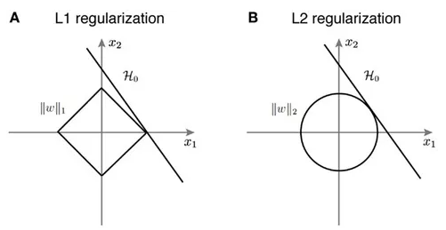
The difference between these priors, and why L1 regularization leads to sparsity, can be beautifully visualized. The MAP estimate is a trade-off between maximizing the likelihood (i.e., minimizing the loss) and satisfying the prior. Geometrically, this is like finding the point on the lowest-level contour of the loss function that is still inside the high-probability region defined by the prior.

Geometric interpretation of L1 and L2 regularization for two parameters, $x_1$ and $x_2$. The ellipses are the level sets of the loss function. The L1 constraint region is a diamond, while the L2 constraint region is a circle.

L2 Regularization (Right): The Gaussian prior $p (\vtheta) \propto exp (- ∣∣ \vtheta ∣ ∣_{2}^{2})$ means that contours of constant prior probability are circles (or hyperspheres in higher dimensions). The loss function's elliptical level sets will most likely touch this circular region at a point where no coordinate is exactly zero.
L1 Regularization (Left): The Laplace prior $p (\vtheta) \propto exp (- ∣∣ \vtheta ∣ ∣_{1})$ means contours of constant prior probability are diamonds (or cross-polytopes). Because of the sharp corners of the diamond lying on the axes, it's much more likely that the expanding ellipses of the loss function will first make contact with the constraint region at one of these corners. A point on a corner has one or more of its coordinates equal to zero. This is the geometric origin of sparsity.

The following video provides an animated walkthrough of this geometric view.

Regularization - Explained!

This video from CodeEmporium provides an excellent visual and conceptual explanation of regularization.

First, watch the geometric explanation of the Ridge constraint, visualizing it as a circular region. Then, see how this changes for the Lasso constraint, which is a diamond shape, making zero-valued coefficients more likely. Finally, the video summarizes the Bayesian connection for both Ridge (Gaussian prior) and Lasso (Laplace prior).

Conclusion

In this lesson, we have elevated our understanding of regularization from a simple "hack" to prevent overfitting to a principled component of Bayesian inference. By moving from MLE to MAP estimation, we've seen how incorporating prior beliefs about model parameters gives a theoretical foundation to the L1 and L2 penalty terms you've likely used countless times.

Key Takeaways:

Maximum a Posteriori (MAP) estimation finds the parameters that maximize the posterior probability $p (\vtheta ∣ X)$ , balancing the likelihood of the data with a prior belief about the parameters.
The MAP objective is equivalent to minimizing the Negative Log-Likelihood (loss) plus a regularization term derived from the negative log-prior, $- lo g p (\vtheta)$ .
Assuming a zero-mean Gaussian prior for the model's weights is equivalent to applying L2 regularization (Ridge).
Assuming a zero-mean Laplace prior for the weights is equivalent to applying L1 regularization (Lasso), which promotes sparsity due to the shape of the prior distribution.

So far, we have focused on finding a single best point estimate for our parameters (either via MLE or MAP). However, a fully Bayesian approach involves reasoning about the entire posterior distribution, not just its mode. This often involves integrals that are analytically intractable. In our next lesson, we will introduce Monte Carlo methods, a powerful set of techniques for approximating these intractable expectations, which are essential for training advanced generative models.

Recommended resources

1. From Likelihood to Posterior Probability

2. Gaussian Priors and L2 Regularization

3. Laplace Priors and L1 Regularization

4. A Geometric Interpretation

Conclusion