Analyzing Iterative Algorithm Complexity

From Exact Counts to Asymptotic Classes

When analyzing an algorithm, one could meticulously count every single operation: every variable assignment, every arithmetic calculation, every array access. This process, while thorough, is incredibly tedious and time-consuming.

Let's look at a resource that demonstrates this. The author of "Analyzing Complexity" from Cornell's CS 2110 course first performs a detailed, line-by-line analysis to find the exact operation count for two algorithms.

As you can see, the final functions are $T(N)=27N+7$ and $T(N)=\frac{11}{2}{N}^2+\frac{7}{2}N+6$. In an interview, nobody expects you to derive these exact formulas. What they do expect is for you to arrive at the asymptotic complexity: $O(N)$ and $O(N^2)$, respectively. Fortunately, we can get there much faster.

The Rules of the Game: Simplified Analysis

Asymptotic notation gives us the power to ignore constant factors and lower-order terms. This leads to two simple but powerful rules for analyzing code:

1. Sequential Blocks: If you have two sequential blocks of code with complexities $O(A)$ and $O(B)$, the total complexity is simply $O(\max (A,B))$. You add the complexities, and the dominant term takes over.
2. Nested Blocks: If a block of code with complexity $O(A)$ is executed $O(B)$ times (e.g., inside a loop), the total complexity is $O(A\cdot B)$. You multiply the complexities.

Let's use these rules to analyze some common patterns.

Constant Time: O(1)

An operation or set of operations is constant time if its execution time does not depend on the input size. This is the holy grail of efficiency.

// O(1) time
int x = 5;
int y = 10;
int sum = x + y;

// Accessing an array element by index is also O(1)
int[] arr = {1, 2, 3, 4, 5};
int thirdElement = arr[2]; // This is O(1) regardless of arr.length

These operations take the same amount of time whether the input array has 5 elements or 5 million. The key is that the number of operations is fixed.

Linear Time: O(n)

This is one of the most common complexities. It occurs when you need to iterate through all elements of a collection once.

// O(n) time
void printAll(int[] arr) {
    System.out.println("Printing elements:");
    for (int i = 0; i < arr.length; i++) { // This loop runs n times
        System.out.println(arr[i]);       // This is an O(1) operation
    }
}

Here, the loop runs arr.length times, which we'll call $n$. Inside the loop, we perform a constant number of operations. Using our rules: the loop body is $O(1)$, and it runs $O(n)$ times. Total complexity: $O(1)\cdot O(n)=O(n)$.

Quadratic Time: O(n²)

Quadratic complexity often arises when you have nested loops iterating over the same data. A classic example is finding if a pair of elements in an array sums to a target value by checking every possible pair.

Let's examine the findPair code from GeeksforGeeks.

The outer loop runs $n$ times, and for each of those iterations, the inner loop also runs $n$ times. This results in $n\times n=n^2$ pairs being checked in the worst case. Total complexity: $O(n)\cdot O(n)=O(n^2)$.

A common variation is a dependent nested loop, where the inner loop's bound depends on the outer loop's variable:

// O(n^2) time
void printPairs(int[] arr) {
    for (int i = 0; i < arr.length; i++) {
        for (int j = i; j < arr.length; j++) { // Inner loop starts from i
            System.out.println(arr[i] + ", " + arr[j]);
        }
    }
}

You might be tempted to think this is faster. And it is! But how much faster? The first time, the inner loop runs $n$ times. The next time, $n-1$, then $n-2$, and so on. The total number of operations is the sum $n+(n-1)+(n-2)+...+1$, which equals $\frac{n(n+1)}{2}=\frac{1}{2}{n}^2+\frac{1}{2}n$. In Big-O notation, we drop the constants and lower-order terms, so this is still $O(n^2)$.

Analyzing Space Complexity

Space complexity measures the amount of extra memory an algorithm needs to run, as a function of the input size. This is often called auxiliary space. We typically don't count the space taken by the input itself.

Constant Space: O(1)

An algorithm uses constant space if it requires a fixed amount of memory, regardless of the input size. In-place algorithms are a great example.

// O(1) space
void reverseArray(int[] arr) {
    int left = 0;
    int right = arr.length - 1;
    while (left < right) {
        // Swap elements
        int temp = arr[left];
        arr[left] = arr[right];
        arr[right] = temp;
        left++;
        right--;
    }
}

This algorithm only uses a few variables (left, right, temp). The number of variables doesn't change whether the array has 10 elements or 10 million. Thus, the auxiliary space is $O(1)$.

Linear Space: O(n)

An algorithm uses linear space if its memory usage grows proportionally to the input size. This often happens when you create a new collection that's a copy of the input or stores related data.

// O(n) space
int[] copyAndDouble(int[] arr) {
    int[] newArr = new int[arr.length]; // Creates a new array of size n
    for (int i = 0; i < arr.length; i++) {
        newArr[i] = arr[i] * 2;
    }
    return newArr;
}

Here, newArr requires space proportional to the size of the input array arr. Therefore, the auxiliary space complexity is $O(n)$.

A very practical example for you as a Java developer involves using HashMap to count frequencies.

Iterative vs. Recursive Space

The distinction between iterative and recursive solutions provides a clear illustration of space complexity. Look at this comparison for calculating a factorial.

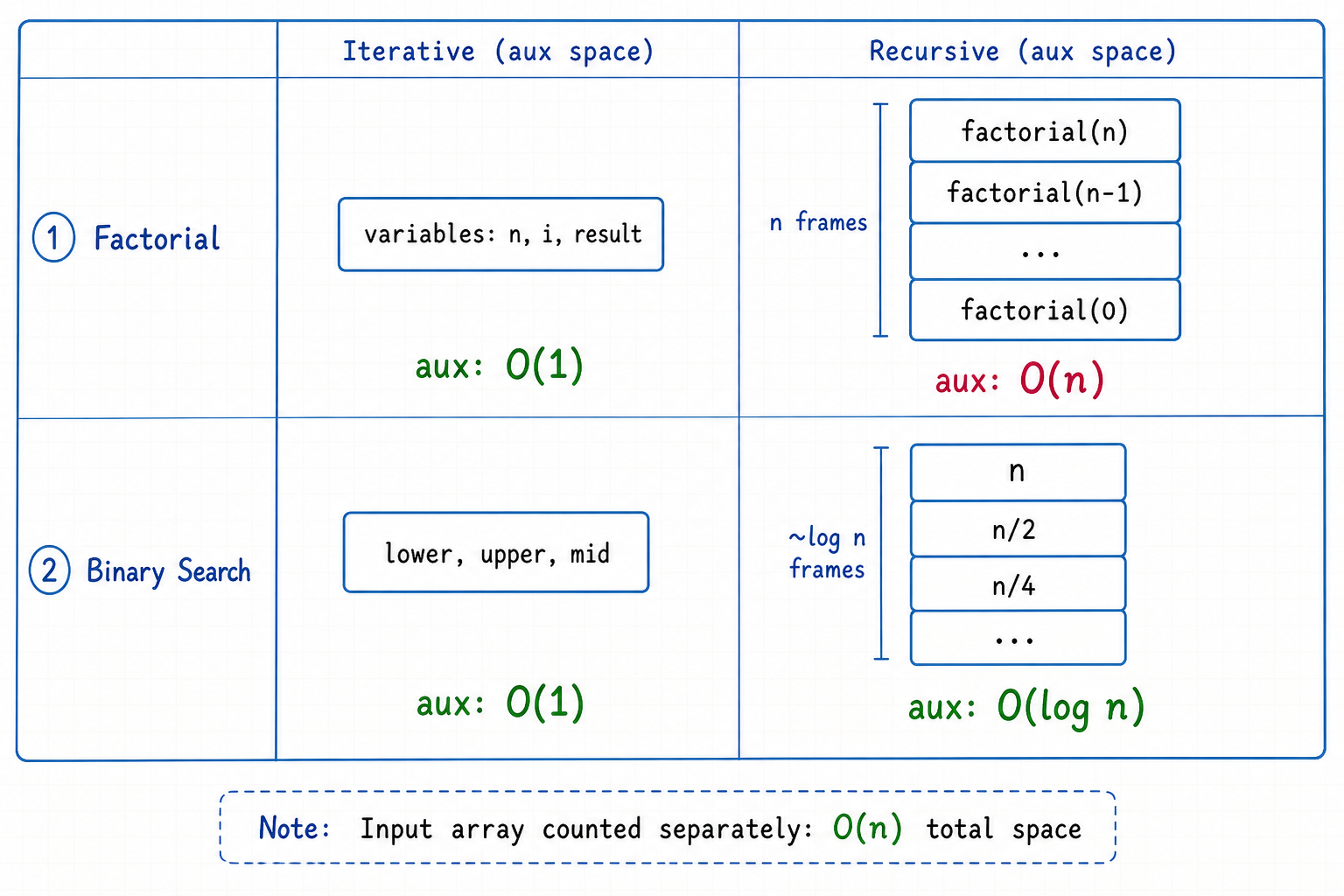
We will cover recursion in depth later, but this visual starkly contrasts the $O(1)$ space of an iterative approach with the $O(n)$ space consumed by the call stack in a naive recursive one.

Visualizing the Difference

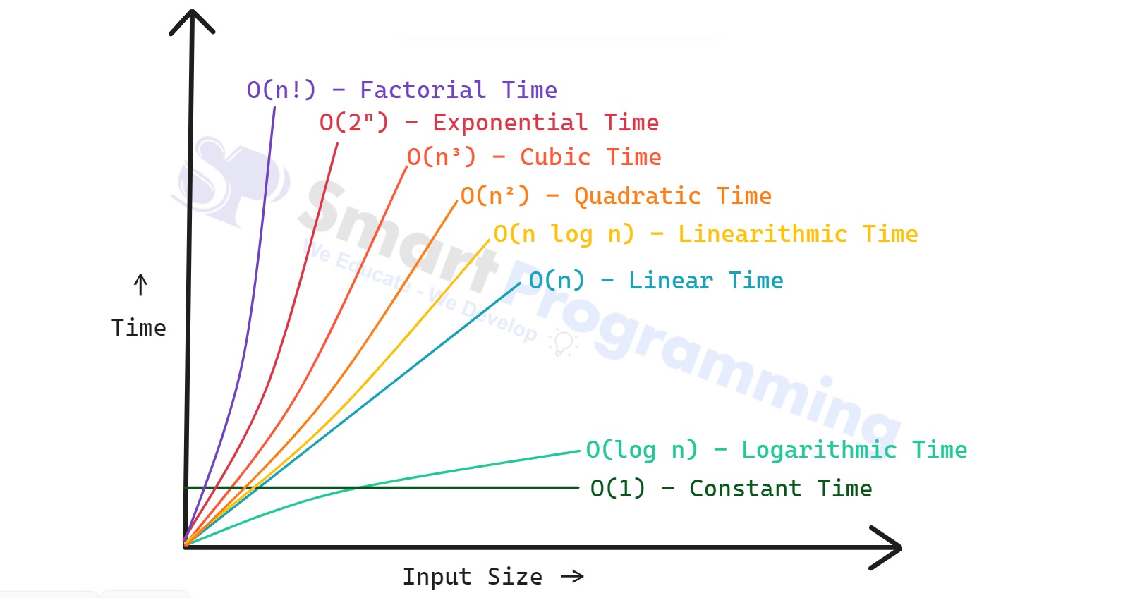
It's one thing to label an algorithm $O(n^2)$, and another to truly appreciate what that means for performance. This graph shows how different complexity classes scale as the input size n increases.

A Final "Gotcha": Java String Concatenation

Because you are a Java developer, it's worth noting a platform-specific detail that can affect complexity analysis. In Java, String objects are immutable. When you concatenate strings in a loop, you aren't just adding to the end of a string; you're creating a new String object in memory each time.

Let's analyze this subtle but important example.

This is a classic interview-style trap. Knowing that s = s + "*" inside a loop of $n$ iterations is an $O(n^2)$ operation in Java demonstrates a deep understanding of both complexity and the language itself.

Conclusion

Today, we've bridged the gap from the theory of asymptotic notation to the practical skill of analyzing code. You now have the mental model to quickly assess the performance of iterative algorithms.

Here are the key takeaways:

• Simplify: Don't count every operation. Use the rules of adding sequential blocks and multiplying nested blocks. The dominant term is all that matters for Big-O.
• Time Complexity Patterns:
  • A simple loop over $n$ elements is typically $O(n)$.
  • A nested loop where both loops go to $n$ is $O(n^2)$.
  • A loop whose counter is repeatedly divided (e.g., i /= 2) is $O(\log n)$. We'll explore this more.
• Space Complexity: This measures the extra memory (auxiliary space) an algorithm uses. $O(1)$ is constant space (in-place), while $O(n)$ is linear space (e.g., creating a copy of an input collection).
• Know Your Language: Language-specific features, like Java's immutable strings, can have surprising performance implications.

In our next lesson, we will take a more structured tour of the common complexity classes you saw on the graph—$O(1)$, $O(\log n)$, $O(n)$, $O(n\log n)$, etc.—and associate each one with a concrete, classic algorithm.