Hello! In our previous lesson, you learned the practical skill of analyzing iterative code to determine its time and space complexity. We saw how a single loop often leads to O(n) complexity, while nested loops can result in O(n²).
Today, we will build on that by taking a systematic tour of the most common complexity classes. Your goal is to develop an intuitive understanding of how these classes compare to one another and to associate each one with a classic algorithmic example. This is crucial for SDE interviews, where you're expected to quickly assess the efficiency of a proposed solution and recognize patterns that could lead to a better one. Think of this as building a mental reference chart of performance trade-offs.
A Visual Hierarchy of Complexity
Before we dive into specifics, let's get a visual sense of what we're comparing. The growth rate of an algorithm's complexity determines how its performance changes as the input size (n) increases. Some algorithms barely feel the change, while others slow to a crawl with even moderately large inputs.
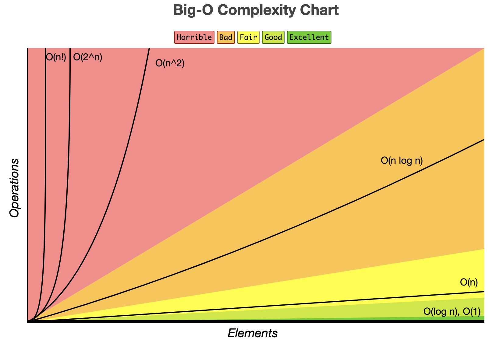
This graph is your map for today's lesson. We'll start in the green "Excellent" zone and work our way up to the red "Horrible" zone. For a deeper, animated perspective on these concepts, the following video provides a great overview.
Big-O Notation - Everything you Need for Coding Interviews
Watch this introductory segment from NeetCode's video "Big-O Notation - Everything you Need for Coding Interviews".
It provides a great conceptual foundation, explaining why we care more about the rate of growth than exact coefficients or constants. Watch from the beginning up to the overview.
Now, let's begin our tour of the main complexity classes.
O(1) — Constant Time: The Gold Standard
An algorithm with O(1) complexity takes the same amount of time to execute, regardless of the input size. These are the most efficient operations.
A prime example is accessing an element in an array by its index. Whether the array has 10 elements or 10 million, myArray[5] takes the same amount of time. Another quintessential example is operations on a hash map.
Big-O Notation - Everything you Need for Coding Interviews
For a concise explanation of constant time, watch this segment on O(1).
The video explains why operations that don't depend on input size are considered constant and uses hash maps as a key example. Watch from the segment on O(1).
Notice the mention of "amortized" time complexity for hash maps. This is an important nuance that we will explore in detail in our next lesson. For now, just know that on average, hash map lookups, insertions, and deletions are O(1).
For a concrete Java example, let's turn to the "Java Challengers" article.
Big (O) Notation Explanation - Java Challengers
This article provides Java code examples for each complexity class.
Read the section on constant time. It shows how simple assignments and array access are O(1).
O(log n) — Logarithmic Time: The Divide and Conqueror
An algorithm with O(log n) complexity is incredibly efficient. As the input size n doubles, the number of operations only increases by one. This happens when the algorithm can repeatedly discard a large fraction (usually half) of the input.
The classic example is Binary Search on a sorted array. By checking the middle element, you can eliminate half of the remaining elements in a single step.
Big-O Notation - Everything you Need for Coding Interviews
To see how this "halving" principle works, watch this segment on O(log n).
Focus on the explanation of how binary search cuts the problem in half with each step. Watch from the O(log n) segment.
Let's see what this looks like in code.
Big (O) Notation Explanation - Java Challengers
Now, read the section on Logarithmic time in the same article.
Focus on the binary search example and its code implementation. Pay attention to how the search space is reduced within the while loop by moving the leftPointer or rightPointer.
O(n) — Linear Time: The Workhorse
This is one of the most common and intuitive complexities. An algorithm with O(n) complexity has a runtime that grows in direct proportion to the input size. If you double the input size, you double the work. This typically occurs when you need to process every element in a collection once.
Big-O Notation - Everything you Need for Coding Interviews
Watch this segment on linear time.
It explains the 1-to-1 growth and uses linear search as a basic example. It also makes an excellent point that nested loops don't automatically mean O(n²), a topic we'll revisit. Watch from the O(n) segment.
Big (O) Notation Explanation - Java Challengers
The article provides a straightforward code example.
Read the linear time section. Note how it clarifies that two separate, non-nested loops over the same input still result in O(n) complexity, not O(2n), because we drop the constant factor.
O(n log n) — Linearithmic Time: The Efficient Sorter
An O(n log n) algorithm performs slightly worse than linear but is still very efficient and scalable. This complexity often arises in "divide and conquer" algorithms that break a problem into smaller subproblems, solve them independently, and then combine the results.
The most famous examples are efficient sorting algorithms like Merge Sort and Quicksort. The intuition is that you are performing an O(log n) operation (splitting the array) for each of the n elements.
Big-O Notation - Everything you Need for Coding Interviews
Now watch the segment on O(n log n) complexity.
The explanation of Merge Sort is particularly clear: there are log n levels of splits, and at each level, n elements are processed. Watch from the O(n log n) segment.
As a Java developer, it's interesting to note that the standard library's sorting methods are highly optimized and typically have this complexity.
Big (O) Notation Explanation - Java Challengers
The article points this out directly.
Read the section on log-linear time. It shows a comment from the JDK source code for Arrays.sort(), confirming its O(n log n) performance.
O(n²) — Quadratic Time: The Nested Loop
An algorithm with O(n²) complexity has a runtime that grows by the square of the input size. If you double the input, the work quadruples. This is a significant performance hit and is often a sign of a brute-force approach. It's typically caused by nested loops that iterate over the same input.
Classic examples include simple sorting algorithms like Bubble Sort, Selection Sort, and Insertion Sort, or any algorithm that needs to compare every element in a collection with every other element.
Big-O Notation - Everything you Need for Coding Interviews
This segment explains the rapid growth of quadratic complexity.
Watch the video's take on O(n²) complexity, which emphasizes its source in nested loops.
Big (O) Notation Explanation - Java Challengers
The code example is a clear illustration.
Read the quadratic section to see the classic double for loop structure.
O(2ⁿ) and O(n!) — Exponential and Factorial Time: The Unscalable
These complexities are in the "Horrible" zone. Their runtime grows so explosively that they are only practical for very small input sizes.
O(2ⁿ) - Exponential Time: The runtime doubles with every single addition to the input. This often appears in recursive algorithms that solve a problem of size n by recursively calling themselves twice on problems of size n-1. A naive recursive solution for computing Fibonacci numbers is a perfect example.
O(n!) - Factorial Time: This is even worse. The runtime grows by a factor of n for each new element. This typically occurs when you need to generate all possible permutations (arrangements) of a set of elements, like in the brute-force solution to the Traveling Salesman Problem.
Big-O Notation - Everything you Need for Coding Interviews
The video provides excellent visualizations for these two classes.
First, watch the explanation for exponential time (O(2^n)), using the Fibonacci example. Then, continue with the segment on factorial time (O(n!)) to understand why it grows even faster.
These "brute-force" complexities are often the starting point in an interview. The challenge is then to find a more clever approach, perhaps using dynamic programming or a different data structure, to reduce the complexity to something more manageable like O(n²) or O(n log n).
The Big Picture: A Cheat Sheet
You've now toured the major complexity classes. It's helpful to see them all laid out in the context of common algorithms and data structure operations. This is exactly what you need to have in your head during an interview.
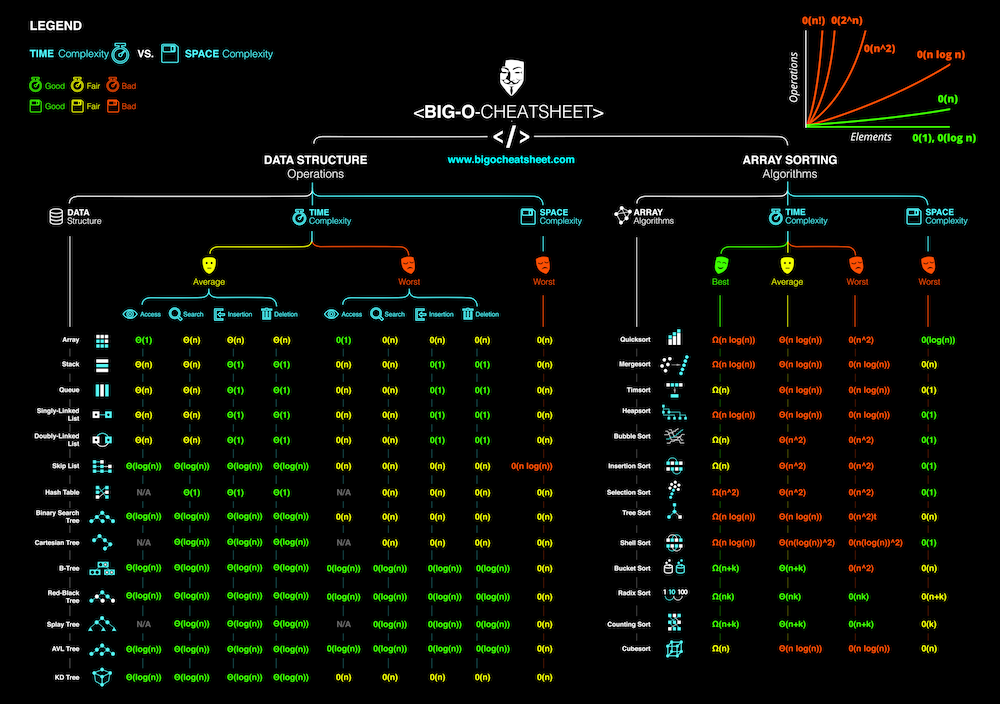
Take a moment to study this image. On the left, notice how operations on a Hash Table are O(1) on average. On the right, see the clear distinction between the O(n²) simple sorts (like Bubble Sort) and the O(n log n) efficient sorts (like Quicksort and Mergesort).
Conclusion
In this lesson, we established a clear hierarchy of common complexity classes and connected each one to a canonical algorithm. This framework is fundamental to algorithmic thinking.
Here are the key takeaways:
- The Hierarchy: The classes we discussed, from best to worst, are: O(1) < O(log n) < O(n) < O(n log n) < O(n²) < O(2ⁿ) < O(n!).
- Recognizing Patterns: You can now associate these complexities with common coding patterns: O(log n) with halving the problem, O(n) with single passes, O(n²) with nested loops, and O(2ⁿ) with certain recursive structures.
- Practical Application: In an interview, when you devise a brute-force solution, you should be able to identify its complexity (e.g., O(n²) or O(2ⁿ)) and then brainstorm ways to improve it by moving down the complexity hierarchy.
In our next lesson, we will do a deep dive into a concept we touched on today: amortized analysis. We will use it to formally explain why operations like adding an element to a dynamic array (like Java's ArrayList) can be considered O(1) on average, even though they sometimes trigger a costly O(n) resize operation.