In our last session, we built a robust toolkit for evaluating classification models, focusing on the trade-offs between metrics like precision, recall, and the specific utility of PR curves for imbalanced data. We now turn our attention from classification to regression, where the goal is to predict a continuous value rather than a discrete class. While the task is different, the need for nuanced evaluation remains just as critical.
This lesson will focus on the three most common and important metrics for regression: Mean Absolute Error (MAE), Root Mean Squared Error (RMSE), and the coefficient of determination (R-squared). As a data scientist, you're already familiar with these in practice. Our goal here is to dissect them mathematically, understand their underlying assumptions, and, most importantly, compare their sensitivities to outliers. This deeper understanding is crucial for both robust model selection and for articulating your modeling choices in a technical interview.
The Foundation: Measuring Individual Errors
At its core, every regression metric is built upon the concept of the residual—the difference between the actual value () and the predicted value () for a single data point.
The challenge is how to aggregate these individual errors across an entire dataset into a single, meaningful number. Do we average them? Do we care more about large errors than small ones? The different metrics we will discuss provide different answers to these questions.
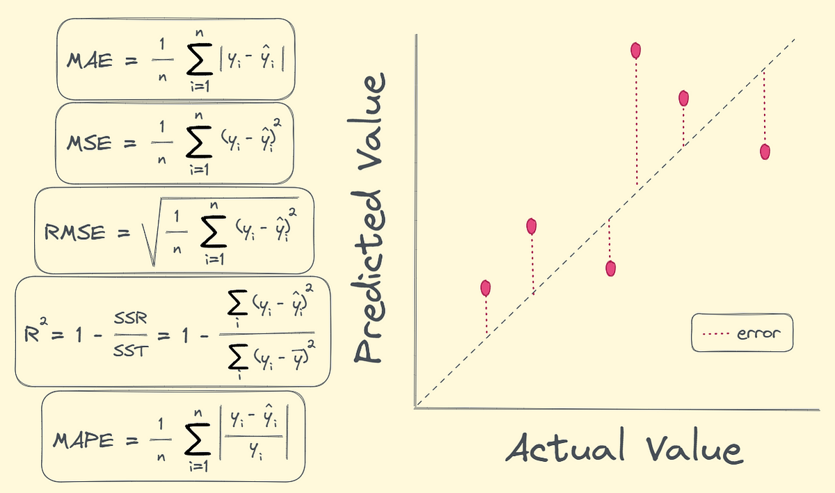
Let's explore the mathematical formulations and practical implications of these different aggregation methods.
Quantifying Average Error: MAE and RMSE
The two most direct ways to measure the average error are the Mean Absolute Error (MAE) and the Root Mean Squared Error (RMSE).
The coefficient of determination R-squared is more ...
This research paper provides concise mathematical definitions for the core regression metrics. We'll use this as our formal reference.
In the "Mathematical background" section, please review the definitions and formulas for: Mean Square Error (MSE) Root Mean Square Error (RMSE) Mean Absolute Error (MAE)
Let's break down the intuition behind these formulas.
-
Mean Absolute Error (MAE):
- Interpretation: MAE measures the average absolute magnitude of the errors. Taking the absolute value prevents positive and negative errors from canceling each other out.
- Units: It is in the same unit as the target variable (e.g., if you're predicting price in dollars, the MAE is in dollars), which makes it highly interpretable. You can say, "on average, our model's prediction is off by X dollars."
-
Mean Squared Error (MSE):
- Interpretation: MSE measures the average of the squared errors. Like MAE, this avoids the cancellation of errors.
- Units: Because of the squaring, the resulting units are also squared (e.g., dollars squared), which is not intuitive. This is a primary reason why we often use its derivative, RMSE.
-
Root Mean Squared Error (RMSE):
- Interpretation: By taking the square root of the MSE, RMSE returns the error metric to the original units of the target variable.
- Units: Like MAE, it is in the same unit as the target variable, making it directly interpretable.
The Crucial Difference: Sensitivity to Outliers
Both MAE and RMSE provide an average error value in the same units, so when would you prefer one over the other? The answer lies in how they treat large errors, or outliers. This is one of the most common points of discussion in technical interviews regarding regression evaluation.
The squaring operation in MSE (and therefore RMSE) gives disproportionately large weight to large errors. A single prediction that is off by 10 units contributes 100 to the sum of squared errors. A prediction off by 2 units contributes only 4. In contrast, MAE treats them linearly (errors of 10 and 2).
This video provides an excellent visual and practical demonstration of this exact point.
Understanding Mean Absolute Error and Mean Squared Error as ML metrics and loss functions
This video from DigitalSreeni clearly explains and demonstrates the different behaviors of MAE and MSE in the presence of outliers.
Please watch two key segments: First, watch the conceptual explanation from the start of the comparison between MAE and MSE. Pay close attention to the graphs that show the linear penalty of MAE versus the quadratic (and rapidly growing) penalty of MSE. Next, watch the Python demonstration starting at the outlier example. The presenter takes a dataset, calculates MAE and MSE, then introduces a single outlier and recalculates. Observe how dramatically the MSE value changes compared to the MAE.
The key takeaways from this comparison are:
- RMSE/MSE is sensitive to outliers. Because it squares the errors before averaging, large errors have a much greater impact on the final metric. You should use RMSE when you want to heavily penalize large errors. This is often the default loss function for regression models for this very reason—it encourages the model to avoid making large mistakes.
- MAE is robust to outliers. It treats all errors with the same linear weight. It is a better choice when you have outliers in your data that you don't want to dominate your evaluation metric.
A useful diagnostic is to compare RMSE and MAE. RMSE will always be greater than or equal to MAE. The larger the difference between them, the greater the variance in your model's errors, which can indicate the presence of significant outliers that are being heavily penalized by RMSE.
Measuring Proportional Fit: R-squared (R²)
While MAE and RMSE tell you the absolute size of the average error, they don't tell you if that error is "good" or "bad" in context. An RMSE of $10,000 might be excellent for a model predicting house prices but terrible for a model predicting the price of a coffee.
R-squared (or the Coefficient of Determination) provides this relative context. It measures the proportion of the variance in the dependent variable that is predictable from the independent variable(s).
The formula is:
Where:
- is the Sum of Squared Residuals (SSR), the error of your model.
- is the Total Sum of Squares (SST), which is proportional to the variance of the actual data. This represents the error of a baseline model that simply predicts the mean value for every point.
Interpretation:
- R² ≈ 1: Your model explains most of the variability in the data. It's a very good fit.
- R² ≈ 0: Your model explains almost none of the variability. It is no better than the simple mean-predicting baseline.
- R² < 0: Your model is worse than the baseline. This can happen with poor models on a test set. This is a critical point to remember.
The following reading explains why a bounded, relative metric like R-squared can often be more informative than an unbounded metric like RMSE or MAE.
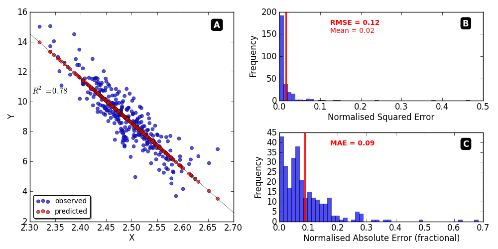
The coefficient of determination R-squared is more ...
This excerpt explains the concept of "informativeness" and why metrics with a fixed range, like R-squared, are easier to interpret without additional context.
In the "Methods" section, read the subsection titled Informativeness. Focus on the argument about why a score like R² = 0.8 clearly indicates good performance, whereas a score like RMSE = 0.7 is meaningless without knowing the scale of the target variable.
Conclusion
You are now equipped to not only calculate but also critically interpret the core regression evaluation metrics. This understanding is key to diagnosing model behavior and selecting the right tool for the job.
Key Takeaways:
- MAE measures the average absolute error. It's robust to outliers and easily interpretable.
- RMSE measures the square root of the average squared error. It is sensitive to outliers, penalizing large errors more heavily. It's often used as a loss function to train models to be cautious of large mistakes.
- R-squared measures the proportion of variance explained by the model compared to a simple mean-based baseline. It provides a context-independent measure of fit. A negative R-squared indicates a model that performs worse than simply predicting the average.
In our next lesson, we will address a fundamental question in model evaluation: how can we be sure our performance metrics are reliable and not just the result of a lucky train-test split? We will explore robust validation strategies, including k-fold, stratified, and time-series cross-validation.