Evaluating Classification Models with Imbalanced Data

The Foundation: The Confusion Matrix

Before any metric can be calculated, we must understand the four possible outcomes of a binary classification prediction. The confusion matrix is a simple table that lays this out clearly. Every classification metric is derived from the values in this matrix.

Let's use a common scenario: a model that predicts whether a transaction is fraudulent (positive class) or legitimate (negative class).

• True Positive (TP): The model correctly predicts a transaction as fraudulent, and it is fraudulent.
• True Negative (TN): The model correctly predicts a transaction as legitimate, and it is legitimate.
• False Positive (FP): The model incorrectly predicts a transaction as fraudulent, but it is actually legitimate. This is a Type I error. Think of this as a false alarm.
• False Negative (FN): The model incorrectly predicts a transaction as legitimate, but it is actually fraudulent. This is a Type II error. This is a missed detection.

To refresh these definitions and see how they are visualized, the following video provides a clear, concise overview.

Core Metrics: The Precision-Recall Tradeoff

With the confusion matrix established, we can define the workhorse metrics of classification. While you're likely familiar with these, the key for both interviews and practice is to articulate their purpose and the inherent tradeoff between them.

The article "Beyond Accuracy" provides an excellent walkthrough of these concepts. We will use it as our guide.

Let's distill the key ideas you've just reviewed:

• Accuracy, $\frac{TP+TN}{Total}$, is misleading for imbalanced data. A model predicting "not fraud" for every transaction in a dataset with 0.1% fraud would have 99.9% accuracy but be completely useless.

• Precision = $\frac{TP}{TP+FP}$

  • Question it answers: "Of all the transactions we flagged as fraud, what fraction were actually fraudulent?"
  • Focus: Minimizing False Positives. High precision is critical when the cost of a false alarm is high (e.g., blocking a customer's legitimate purchase, flagging a critical email as spam).

• Recall (or Sensitivity, True Positive Rate) = $\frac{TP}{TP+FN}$

  • Question it answers: "Of all the actual fraudulent transactions, what fraction did we successfully catch?"
  • Focus: Minimizing False Negatives. High recall is critical when the cost of a missed detection is high (e.g., failing to detect cancer, letting a fraudulent transaction go through).

There is a fundamental tradeoff between precision and recall. If you want to increase recall (catch more fraud), you can lower your model's prediction threshold. This means more transactions get flagged, catching more true fraud but also inevitably flagging more legitimate transactions as fraudulent (lowering precision).

• F1-Score = $2\times \frac{\text{Precision}\times \text{Recall}}{\text{Precision}+\text{Recall}}$
  • The harmonic mean of precision and recall. The key property of the harmonic mean is that it is heavily penalized by low values. A model must have both decent precision and recall to achieve a high F1-score. This makes it a more reliable summary metric for imbalanced classes than accuracy.

Evaluating Performance Across All Thresholds: ROC and AUC

Precision, recall, and F1-score are all calculated for a single classification threshold (e.g., if predicted probability > 0.7, classify as fraud). However, a model's real strength is its ability to rank cases, with fraudulent transactions hopefully getting higher scores than legitimate ones. The Receiver Operating Characteristic (ROC) curve helps us evaluate this ranking power across all possible thresholds.

The ROC curve plots True Positive Rate (Recall) on the y-axis against False Positive Rate (FPR) on the x-axis, where $\text{FPR}=\frac{FP}{FP+TN}$.

• The curve is generated by sweeping the classification threshold from 1 down to 0.
• An ideal model's curve hugs the top-left corner (TPR=1, FPR=0).
• A diagonal line from (0,0) to (1,1) represents a model with no discriminative power (random guessing).

The Area Under the ROC Curve (ROC-AUC) summarizes this plot into a single number.

• AUC = 1.0: A perfect classifier.
• AUC = 0.5: A classifier no better than random chance.

The most important interpretation of AUC, especially for an interview setting, is its probabilistic meaning: The AUC is the probability that a randomly chosen positive example is ranked higher by the classifier than a randomly chosen negative example.

This directly connects to a non-parametric statistical test, the Mann-Whitney U test, which tests whether two samples come from the same distribution. This connection reveals that AUC is fundamentally a measure of rank-ordering quality.

The Pitfall of ROC-AUC in High Imbalance

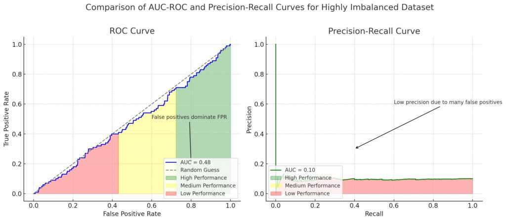
While ROC-AUC is better than accuracy for imbalanced data, it can still paint an overly optimistic picture in cases of extreme imbalance.

Why? Look at the False Positive Rate formula: $\text{FPR}=\frac{FP}{FP+TN}$. In a dataset with 99.9% legitimate transactions (negatives), the denominator ($FP+TN$) is massive. Even if the model makes thousands of false positive predictions, the FPR can remain very low simply because the number of true negatives is so large. This can make the ROC curve look deceptively good.

The following video does an excellent job of explaining this limitation and introduces the preferred alternative.

The Solution: Precision-Recall (PR) Curves

When dealing with highly imbalanced datasets where the positive class is your primary interest, the Precision-Recall (PR) Curve is a more informative tool.

• It plots Precision (y-axis) vs. Recall (x-axis).
• Since both precision and recall are calculated using TP, FP, and FN, the metric is not "propped up" by the vast number of TNs. It focuses entirely on the model's performance on the challenging positive class.
• An ideal model's PR curve hugs the top-right corner (Precision=1, Recall=1).
• The baseline for a PR curve is not 0.5; it is the fraction of positives in the dataset (e.g., for a dataset with 1% positives, the baseline is 0.01). A model that significantly outperforms this baseline is doing well.

The Area Under the PR Curve (PR-AUC) gives a single-number summary. A high PR-AUC on an imbalanced dataset is a strong indicator of a high-quality model.

Choosing the Right Metric: A Practical Framework

So, which metric should you use? The answer always depends on the business context and the relative costs of Type I and Type II errors.

Here is a summary that aligns with this flowchart:

• Is the data balanced and are error costs equal? -> Accuracy and ROC-AUC are fine.
• Is the data imbalanced?
  • Is the cost of False Negatives high? (e.g., fraud, disease detection) -> Prioritize Recall.
  • Is the cost of False Positives high? (e.g., spam filter, flagging innocent users) -> Prioritize Precision.
  • Are both error types costly? -> Use F1-Score for a balanced view at a specific threshold.
  • Do you want to evaluate overall model performance on a highly imbalanced dataset where the positive class is key? -> Use the PR Curve and PR-AUC.

For a final review, and to prepare for interviews, the "Beyond Accuracy" article has an excellent summary guide and a list of common interview questions.

Conclusion

You now have a comprehensive framework for evaluating classification models that goes far beyond simple accuracy.

Key Takeaways:

• Accuracy is a poor choice for imbalanced datasets.
• The choice between prioritizing Precision (minimizing FPs) and Recall (minimizing FNs) is a business decision based on error costs. The F1-score balances this tradeoff.
• ROC-AUC measures a model's ability to rank positive and negative examples and is a good general-purpose metric, but it can be misleadingly optimistic on highly imbalanced data.
• The Precision-Recall (PR) curve and its AUC provide a more truthful assessment of model performance on highly imbalanced datasets, especially when the minority positive class is the focus.

In our next lesson, we'll complete our tour of fundamental evaluation techniques by examining metrics for regression models, such as RMSE, MAE, and R-squared, and analyzing their sensitivity to outliers.