Time-Series Forecasting with Recurrent Models

1. The Challenge of Sequential Data

Standard feedforward networks, like the perceptrons we've discussed, treat each input as an independent event. However, in time-series data—like stock prices, weather patterns, or sensor readings—the order of events is paramount. The value at time $t$ is often dependent on the values at $t-1,t-2,\dots$. To capture these temporal dependencies, we need a new kind of architecture.

Recurrent Neural Networks (RNNs) solve this by introducing a "memory" or an internal state, typically denoted as $h_t$. This state is updated at each time step and carries information from the past into the present computation.

The key insight is the recurrence relation:

The state at the current time step, $h_t$, is a function of both the current input $x_t$ and the previous state $h_{t-1}$. This simple loop is what gives RNNs their ability to "remember" and process sequences.

2. Framing the Forecasting Problem

Before we can feed data into an RNN, we must structure it in a way the model can understand. This involves framing our time series task into a supervised learning problem with clear inputs (X) and targets (y). The way we do this depends on the specific question we're asking.

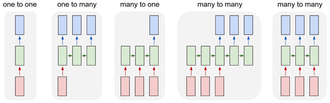
• Many-to-One: We use a sequence of past values to predict a single future value. For example, using the last 30 days of a stock's price to predict tomorrow's price.
• Many-to-Many: We use a sequence of past values to predict a sequence of future values. For example, using the last week's weather data to predict the forecast for the next three days.

The fundamental technique for creating these structures is the sliding window or lookback method.

3. The Sliding Window: Creating Input/Output Pairs

The "lookback" defines how many previous time steps the model gets to see to make a prediction. We slide this window across our time series to generate multiple input-output samples.

A fantastic article from Machine Learning Mastery demonstrates this with a classic dataset: predicting airline passenger numbers. The core logic is encapsulated in a single, powerful function.

Let's trace the logic with a simple example. Imagine our time series is [10, 20, 30, 40, 50, 60] and we set lookback = 3. The create_dataset function would generate the following pairs:

1. Input X: [10, 20, 30], Target y: [20, 30, 40]
2. Input X: [20, 30, 40], Target y: [30, 40, 50]
3. Input X: [30, 40, 50], Target y: [40, 50, 60]

The function from the article creates input and target sequences of the same length. This is a common setup for a "many-to-many" task where the model learns to predict the next value at each time step. The final prediction we care about for forecasting is often the last element of the output sequence.

The result is a dataset where each sample X is a sequence of length lookback, and each y is the corresponding future sequence. When batched together, the input tensor X will have the shape (batch_size, sequence_length, num_features), which is exactly what PyTorch's recurrent layers expect when configured with batch_first=True.

4. A Concrete Implementation in PyTorch

Now let's see how this data structuring is implemented within a complete PyTorch workflow. The following article from Towards Data Science walks through building an LSTM to learn a sine wave, and its data preparation and forward pass logic are highly instructive.

This approach demonstrates two key ideas:

1. Teacher Forcing during Training: By providing the full input and target sequences (y[:, :-1] and y[:, 1:]), we are "forcing" the model at each step with the correct ground-truth value from the previous step. This stabilizes training.
2. Autoregressive Generation during Inference: To predict the future, the model uses its own prediction for time $t$ as part of the input to predict time $t+1$.

5. Integrating with PyTorch's Dataset and DataLoader

The final step is to wrap this data generation logic in a PyTorch Dataset class. This allows PyTorch's DataLoader to efficiently handle batching, shuffling, and parallel data loading.

Using a custom Dataset makes your code modular and clean. The logic for creating windows is contained within the dataset, and your training loop simply iterates over the DataLoader.

6. An Expert Distinction: Evaluation vs. True Forecasting

As you move towards a senior engineering role, it's vital to understand a subtle but critical distinction in how time-series models are evaluated. The code in the Machine Learning Mastery article plots model(X_test). A sharp reader pointed out a potential issue with this, leading to an excellent clarification.

Understanding this difference is what separates a practitioner who can train a model from an engineer who can deploy a reliable forecasting system. Your approach to evaluation must match the intended use case.

Conclusion

In this lesson, you've learned the fundamental principles of preparing data for recurrent models. This is a non-trivial but essential step in the pipeline for any sequential task.

Key Takeaways:

• Time-series forecasting requires structuring a flat sequence of data into input/output pairs using a sliding window (or "lookback") method.
• The shape of your problem—predicting one step (many-to-one) or many steps (many-to-many)—determines how you define your target sequences.
• The standard tensor format for PyTorch recurrent layers is (batch_size, sequence_length, num_features).
• PyTorch's Dataset class is the ideal place to implement your windowing logic, keeping your data preparation modular and efficient.
• There is a critical difference between evaluating a model with ground-truth inputs (teacher forcing) and simulating real-world autoregressive forecasting, where the model relies on its own past predictions.

We've focused on how to structure data for models that read sequences. In the next lesson, we will pivot to a different type of data and architecture by exploring the mechanics of the 2D convolution operation, the workhorse behind models that "see" grid-like data such as images.