Understanding 2D Convolution: Kernels, Padding, and Stride

Welcome back. In our previous lesson, we focused on structuring data for models that process information sequentially, like RNNs. You learned to use the sliding window technique to transform a 1D time series into the (batch, sequence, features) format that recurrent models expect.

We now pivot from the temporal dimension to the spatial dimensions. Instead of data where order over time is key, we'll explore data with a grid-like structure, such as images. This requires a different architectural primitive: the convolution. Your goal for this lesson is to explain the mechanics of a 2D convolution operation, detailing the roles of kernels, padding, and stride. Mastering this is not just about understanding computer vision; it's about grasping a fundamental computational block that appears in many modern architectures.

1. From Sequential to Spatial: The Need for Convolutions

A fully connected network processing a moderately sized 200x200 pixel image would require neurons with 120,000 weights each in the first layer—an unmanageable number that leads to massive computational cost and overfitting. Recurrent networks are designed for sequences, not spatial hierarchies.

Convolutional Neural Networks (CNNs) solve this by using a more sensible architecture for image-like data. Instead of connecting every neuron to every other, they use a principle of local connectivity.

https://cs231n.github.io/convolutional-networks/

This foundational text from Stanford's CS231n course provides an excellent overview of why CNNs are necessary and how they are structured.

First, read the introduction and "Architecture Overview" to understand the problem with applying regular neural networks to images. Focus on the concept of arranging neurons in 3D volumes (width, height, depth). Next, read the section "Convolutional Layer" up to "Local Connectivity." Pay close attention to the intuitive explanation of a filter. The core idea is that a filter is a small, learnable pattern detector that slides across the input.

The key takeaways are:

Locality: A neuron in a convolutional layer is only connected to a small, local region of the input (its receptive field).
Parameter Sharing: A single filter (a set of weights) is used across all spatial locations of the input. If a horizontal edge detector is useful in the top-left of an image, it's likely useful elsewhere too. This drastically reduces the number of parameters.
3D Tensors: Layers in a CNN transform a 3D input volume (e.g., width x height x channels) to a 3D output volume.

2. The Mechanics of the 2D Convolution

The term "convolution" in deep learning refers to an operation where a kernel (or filter) slides over the input tensor. At each position, an element-wise multiplication between the kernel's values and the overlapping input patch is performed, and the results are summed to produce a single output pixel.

Most 2D animations of this process are misleading because they ignore the depth dimension. In practice, we operate on 3D volumes.

All Convolution Animations Are Wrong (Neural Networks)

The creator of this video, Grant Sanderson (of 3Blue1Brown fame), highlights why typical 2D convolution animations are insufficient and presents a more accurate 3D visualization.

Watch the entire video. Pay attention to how it contrasts simplified 2D animations with a more accurate 3D representation (the problem). Then, carefully observe the correct 3D animation (the solution). Notice three crucial details: The input is a 3D volume (e.g., width, height, 3 color channels). The filters are also 3D volumes; their depth must match the input depth. Each filter produces one 2D slice (an activation map) of the output. The number of filters determines the depth of the output volume.

The convolution operation itself is governed by three primary hyperparameters that control the geometry of the output: padding, stride, and the number of filters (which determines output depth).

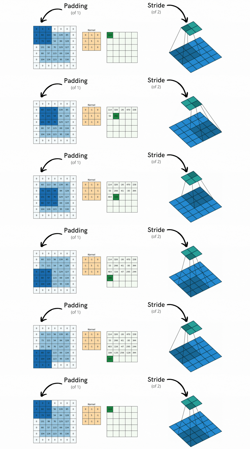
This animation illustrates the core mechanics of padding (adding a border of zeros) and stride (the step size of the kernel). These hyperparameters give us precise control over the output tensor's spatial dimensions.

Hyperparameters: Stride and Padding

Stride dictates how many pixels the kernel "jumps" as it slides across the input.

A stride of 1 moves the filter one pixel at a time, resulting in a densely computed output.
A stride of 2 skips every other pixel, effectively downsampling the input by a factor of approximately 2 in each spatial dimension.

Padding involves adding a border of zeros around the input tensor before the convolution. It serves two main purposes:

Preserving Spatial Dimensions: Without padding, each convolution would shrink the spatial dimensions. By adding padding, we can ensure the output has the same width and height as the input. A common rule of thumb is to use padding = (kernel_size - 1) / 2 for a stride of 1.
Improving Border Processing: Padding allows the kernel to be centered on pixels at the edge of the original image, ensuring they are processed as thoroughly as the central pixels.

The spatial dimensions of the output can be calculated with a simple formula. For an input of width $W$ , a kernel of size $F$ , padding $P$ , and stride $S$ , the output width $W_{o u t}$ is:

W_{o u t} = \frac{W - F + 2 P}{S} + 1

This formula is fundamental to designing CNN architectures, as it allows you to reason about how the tensor shapes evolve through the network.

https://cs231n.github.io/convolutional-networks/

This section of the CS231n notes formalizes the concepts of stride and padding and provides the definitive formula for output size.

Read the section on Spatial arrangement. Focus on understanding the roles of depth, stride, and zero-padding, and how they relate to the output size formula. The graphical example of stride is particularly helpful.

3. From Scratch: Implementing `conv2d` in NumPy

To truly understand the mechanics, we will implement the operation from scratch. This moves beyond API consumption and forces a confrontation with the underlying loops and array manipulations.

The article "Convolutional Neural Networks from Scratch" provides a clear NumPy implementation that we can analyze.

Convolutional Neural Networks from Scratch: Building Conv2d with NumPy

This article demystifies the Conv2d layer by building it from scratch in NumPy, providing a direct comparison to PyTorch's implementation.

First, read the section "The Convolution Operation" to see the core element-wise multiplication and summation. Next, study the conv2d_numpy function in the section "Building Conv2d from Scratch". This function, with its nested loops, is the most explicit representation of the sliding window operation. Note how the loop indices and slicing (h_start, w_start, patch) directly implement the concepts of stride and kernel application. Finally, and most importantly, examine the conv2d_multichannel function under the section "Multi-Channel Convolution". This is the correct implementation for real-world use. Notice the additional loops for input channels (ci) and output channels (co). For each output channel, the code convolves the corresponding filter over all input channels and sums the results. This is the mechanism that mixes information across channels.

Verifying that your from-scratch NumPy code produces the exact same output as torch.nn.functional.conv2d is a powerful confirmation of understanding. The core logic is identical; the difference lies in the highly optimized C++/CUDA backend used by frameworks like PyTorch.

4. A Point of Precision: Convolution vs. Cross-Correlation

In the deep learning community, the term "convolution" is used to describe the sliding dot-product operation we've discussed. However, from a signal processing and mathematical standpoint, this operation is technically cross-correlation. True convolution requires rotating the kernel by 180 degrees before applying it.

Convolutional Neural Network from Scratch | Mathematics & Python Code

This video provides a clear mathematical breakdown of the forward and backward passes of a convolution layer. We will focus on its precise definition of terms.

Watch the initial segment from convolution vs. cross-correlation. This clarifies the formal difference. In deep learning, since the kernel's weights are learned via backpropagation, the distinction is academic. The network will simply learn the appropriately rotated kernel if needed. Nonetheless, knowing this distinction is a mark of a careful engineer.

5. The Performance Trick: `im2col`

The nested-loop implementation is intuitive but computationally inefficient. Modern deep learning libraries achieve high performance by transforming the convolution into a single, large matrix multiplication (GEMM), for which highly optimized libraries (like BLAS) exist. This transformation is commonly called im2col (image-to-column).

The im2col operation works as follows:

It extracts every local patch from the input image that the kernel will operate on.
It "unrolls" or "stretches" each of these 3D patches into a single column vector.
All these column vectors are stacked side-by-side to form a large matrix.
The convolution filters are also unrolled into rows of another matrix.
The entire convolution for all filters across all positions can now be computed with a single matrix multiplication between the filter matrix and the im2col input matrix.

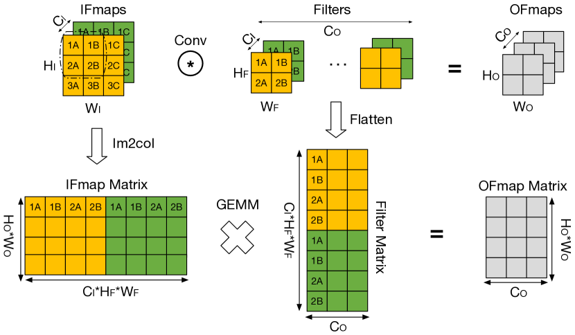
This diagram illustrates the im2col transformation. The input feature map (IFmap) is unrolled into a matrix where each column is a receptive field. The filters are flattened into rows of a filter matrix. The convolution is then performed as a General Matrix Multiplication (GEMM), which is highly optimized on modern hardware.

This is a crucial optimization that underpins the practical performance of CNNs. While it comes at the cost of increased memory usage (as pixel values are duplicated in the im2col matrix), the computational speedup is substantial.

Conclusion

In this lesson, you've dissected the 2D convolution operation, the fundamental building block for processing grid-like data. You have moved from a high-level intuition to a from-scratch implementation and an understanding of the performance optimizations used in production libraries.

Key Takeaways:

Core Mechanic: A 2D convolution is a sliding dot-product operation where a learnable kernel detects features in local regions of an input tensor.
3D Volumes: The operation transforms a 3D input volume to a 3D output volume. The filter depth must match the input depth, and the number of filters determines the output depth.
Hyperparameters: Stride controls the step size and downsampling, while padding controls the border and output spatial size. The output dimensions are governed by a predictable formula: $W_{o u t} = (W - F + 2 P) / S + 1$ .
Parameter Sharing: Using the same kernel across all spatial locations dramatically reduces the number of learnable parameters and encodes an assumption of translational invariance.
Efficiency: While conceptually a series of nested loops, efficient convolution is implemented as a single large matrix multiplication via the im2col transformation.

With this foundational piece in place, you are ready to understand how these layers are trained. In the next module, we will begin our exploration of "Advanced Training and Optimization," starting with the construction of a custom PyTorch training loop from scratch to train the very parameters (kernels) we've just discussed.

Recommended resources