Eigenvalues, Eigenvectors, and SVD for Model Analysis & Low-Rank Approximation

1. Eigenvectors and Eigenvalues: The Skeletons of a Transformation

A linear transformation, represented by a matrix, can stretch, squish, rotate, and shear vectors in space. Amidst this complex motion, certain vectors stand out. These special vectors, called eigenvectors, are those that are not knocked off their original span by the transformation. Their direction remains unchanged; they are only scaled. The factor by which they are scaled is their corresponding eigenvalue, denoted by $\lambda$.

This concept provides a powerful way to understand a transformation's fundamental behavior by identifying its "axes" of action.

Formally, for a square matrix $A$, a non-zero vector $\mathbf{v}$ is an eigenvector if it satisfies the equation:

where $\lambda$ is the scalar eigenvalue. This equation states that the action of the matrix $A$ on the vector $\mathbf{v}$ is the same as simply scaling $\mathbf{v}$ by $\lambda$.

To find these, we can rearrange the equation:

For this equation to have a non-zero solution for $\mathbf{v}$, the matrix $(A-\lambda I)$ must be singular, meaning it squishes space into a lower dimension. This is equivalent to its determinant being zero:

Solving this characteristic equation gives us the eigenvalues $\lambda$. We can then plug each $\lambda$ back into $(A-\lambda I)\mathbf{v}=0$ to solve for the corresponding eigenvectors $\mathbf{v}$.

While powerful, eigenvalue decomposition has a major limitation: it only applies to square matrices. This is where SVD comes in.

2. Singular Value Decomposition (SVD): A Generalization for All Matrices

The Singular Value Decomposition (SVD) is one of the most important factorizations in linear algebra. It asserts that any $m\times n$ matrix $A$ can be decomposed into three component matrices:

where:

• $U$ is an $m\times m$ orthogonal matrix whose columns are the left-singular vectors.
• $\Sigma$ is an $m\times n$ diagonal matrix with non-negative, sorted values ${\sigma }_1\ge {\sigma }_2\ge ...\ge 0$ on its diagonal. These are the singular values.
• $V^T$ is the transpose of an $n\times n$ orthogonal matrix $V$, whose columns are the right-singular vectors.

Geometrically, SVD states that any linear transformation can be broken down into a sequence of three fundamental operations: a rotation (or reflection) by $V^T$, a scaling along the axes by $\Sigma$, and another rotation (or reflection) by $U$.

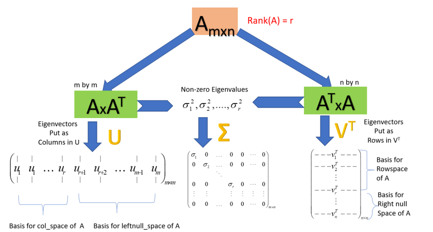
The critical insight for your work is how SVD connects to eigenvalues. Since $A$ can be rectangular, we can't find its eigenvalues directly. However, we can construct two related square, symmetric matrices: $A^{T}A$ and $A{A}^T$. These matrices are always positive semidefinite, guaranteeing their eigenvalues are real and non-negative.

The connection is profound:

1. The columns of $V$ (the right-singular vectors of $A$) are the eigenvectors of $A^{T}A$.
2. The columns of $U$ (the left-singular vectors of $A$) are the eigenvectors of $A{A}^T$.
3. The non-zero singular values of $A$ (${\sigma }_i$) are the square roots of the non-zero eigenvalues of both $A^{T}A$ and $A{A}^T$. (${\sigma }_i=\sqrt{{\lambda }_i}$).

3. Application 1: Low-Rank Approximation

The SVD provides a decomposition of a matrix into a sum of rank-1 matrices, ordered by importance via the singular values:

where $r$ is the rank of $A$, and ${\mathbf{u}}_i,{\mathbf{v}}_i$ are the $i$-th singular vectors.

Many real-world matrices, including weight matrices in neural networks, are "compressible" in the sense that their essential information is captured by the first few, largest singular values. The remaining singular values are small and can be discarded with minimal loss of information.

This leads to low-rank approximation. By keeping only the top $k$ singular values and their corresponding vectors, we can construct a new matrix $A_k$ that is the best possible rank-$k$ approximation of $A$ (in the Frobenius norm sense, as guaranteed by the Eckart-Young-Mirsky theorem).

This is not just a compression trick. It's a foundational technique for efficiency in modern AI.

A classic visual example is image compression. An image can be represented as a matrix of pixel values. By performing a low-rank approximation via truncated SVD, we can drastically reduce the amount of data needed to store the image while preserving most of the visual content.

4. Application 2: Model and Data Analysis (PCA)

Beyond approximation, SVD is the engine behind Principal Component Analysis (PCA), a cornerstone of data analysis. PCA seeks to find the directions of maximum variance in a dataset—the "principal components."

Given a data matrix $X$ where each row is a data point, the principal components are precisely the eigenvectors of the covariance matrix $X^{T}X$. As we established earlier, the eigenvectors of $X^{T}X$ are the right-singular vectors of $X$ (the columns of $V$, or rows of $V^T$).

Therefore, computing the SVD of your data matrix $X$ directly gives you the principal components. The singular values ${\sigma }_i$ are related to the amount of variance captured by each component, so they tell you which components are most important for describing the data.

In the context of AI, you can apply this to analyze weight matrices, activation patterns, or embedding spaces to understand the dominant "concepts" or features learned by a model.

Conclusion

In this lesson, we transitioned from the calculus of optimization to the linear algebra of structure. You've now equipped yourself with a set of powerful analytical tools that are central to modern AI engineering.

The key takeaways are:

• Eigenvectors and eigenvalues reveal the intrinsic axes of a linear transformation, showing directions that are purely scaled.
• Singular Value Decomposition (SVD) generalizes this idea to any matrix ($A=U\Sigma V^T$), breaking it down into rotation, scaling, and rotation.
• The components of SVD are deeply connected to eigenvalues: the singular vectors of $A$ are the eigenvectors of $A^{T}A$ and $A{A}^T$.
• Low-rank approximation via truncated SVD is the optimal way to compress a matrix, forming the theoretical basis for techniques like LoRA.
• SVD is the computational engine behind PCA, allowing you to find the most significant patterns and directions of variance in your data or model components.

You now have the necessary calculus and linear algebra foundations. In our next lesson, we will add the third pillar of our mathematical toolkit: probability. We will explore the probabilistic interpretation of common loss functions like Cross-Entropy, connecting them to the principle of maximum likelihood estimation. This will give you a deeper understanding of why we choose certain objective functions when training our models.