Welcome to the third lesson in our "Mathematical Toolkit" module. So far, we have covered the calculus of optimization through backpropagation and the linear algebra of structure with SVD. We now add the third and final pillar to our mathematical foundation: probability. Your goal is to understand AI systems "under the hood," and this involves knowing why we choose certain loss functions. They are not arbitrary; they are deeply rooted in probabilistic principles.
In this lesson, you will learn the probabilistic interpretation of common loss functions. We will demystify terms like Cross-Entropy and show their direct connection to the fundamental statistical principle of Maximum Likelihood Estimation (MLE). By the end, you'll be able to explain not just what these loss functions do, but why they are the right tool for the job from a first-principles perspective.
1. The Principle of Maximum Likelihood Estimation (MLE)
At its core, training a supervised machine learning model is a search problem. We are searching for the set of model parameters, , that best explains the data we've observed. The principle of Maximum Likelihood Estimation (MLE) formalizes this. It directs us to choose the parameters that maximize the probability—or more accurately, the likelihood—of observing our training dataset.
Given a set of independent and identically distributed (i.i.d.) data points , the likelihood of the entire dataset is the product of the probabilities of each individual data point:
Here, is the probability of observing label given input , according to our model with parameters .
Working with products is computationally difficult and can lead to numerical underflow. It's much easier to work with sums. Since the logarithm is a monotonically increasing function, maximizing the likelihood is equivalent to maximizing the log-likelihood:
Most optimization frameworks are designed to minimize a loss function. Therefore, we can frame our goal as minimizing the negative log-likelihood (NLL):
This simple reframing is the bridge between statistical estimation and the loss functions you encounter in deep learning.
This article provides an excellent conceptual bridge between familiar ML models and their statistical underpinnings. The author's journey from "scikit-learn fit and predict" to understanding the 'why' mirrors your own goals.
Start by reading the section on Maximum likelihood estimation. Focus on the derivation that connects maximizing the likelihood over a dataset to minimizing the final loss function. This will show you exactly how Mean Squared Error, Binary Cross-Entropy, and Categorical Cross-Entropy emerge from the NLL principle when applied to different probability distributions (Gaussian, Binomial, and Multinomial, respectively).
2. Example: Why Mean Squared Error is a Negative Log-Likelihood
Let's make this concrete with a familiar loss function: Mean Squared Error (MSE). You've likely used it for regression tasks, but why is it the standard choice? The answer lies in MLE.
For a regression problem, we often implicitly assume that our target variable is a combination of our model's deterministic prediction and some random Gaussian noise , where . This is equivalent to assuming that the probability of observing a specific given follows a Gaussian (normal) distribution centered at our model's prediction:
The probability density function (PDF) for a single point is therefore:
The negative log-likelihood for a single data point is:
To find the parameters that maximize the likelihood for the entire dataset, we minimize the sum of NLL over all points. When we do this, the first term, , is a constant with respect to . The in the denominator is also a constant scaling factor. Therefore, minimizing the NLL is equivalent to minimizing:
This is precisely the Mean Squared Error loss (ignoring the constant factor ). This derivation shows that using MSE is equivalent to performing maximum likelihood estimation under the assumption of Gaussian noise.
GLM Intro - 2 - Least Squares vs. Maximum Likelihood
This video provides a great visual and mathematical walkthrough of the equivalence between Least Squares (which MSE minimizes) and Maximum Likelihood.
Watch from the start of the comparison to understand the core assumption that the data points are normally distributed around the regression line. Then, follow the derivation from the likelihood function to see how maximizing the log-likelihood for a normal distribution simplifies to minimizing the sum of squared errors.
3. Cross-Entropy and KL Divergence: Measuring the Distance Between Distributions
While the Gaussian assumption works for regression, it's unsuitable for classification, where outputs are discrete class labels. In classification, our model outputs a probability distribution (via softmax), and our goal is to make this distribution as "close" as possible to the true distribution (which is a one-hot vector representing the correct class).
Information theory provides the tools to measure this "closeness":
- Cross-Entropy: Suppose the true data distribution is and our model's predicted distribution is . The cross-entropy, , measures the average number of bits required to encode data from when using a code optimized for . The formula is:
- Kullback-Leibler (KL) Divergence: This measures the extra bits required because we used the "wrong" distribution instead of the true one . It's a measure of how much diverges from . where is the entropy of the true distribution. Since is a constant with respect to our model's parameters, minimizing the KL divergence is equivalent to minimizing the cross-entropy.
Training a classification model is therefore an exercise in minimizing the KL divergence between the true data distribution and our model's predicted distribution .
This chapter from Classical Foundations of Artificial Neural Networks provides the rigorous definitions and proofs you need. It connects the ideas of Shannon, Kullback, and Leibler directly to neural network loss functions.
Read the section Cross-Entropy and KL Divergence. Pay close attention to the definitions of Cross-Entropy and KL Divergence. Crucially, understand the proof for Theorem 26.3, which formally shows that minimizing cross-entropy is equivalent to minimizing KL divergence.
4. The Unifying Trinity: MLE, KL Divergence, and Cross-Entropy
We have now established two key equivalences:
- Minimizing Negative Log-Likelihood Maximum Likelihood Estimation.
- Minimizing Cross-Entropy Minimizing KL Divergence.
The final step is to connect these two worlds. It turns out that performing Maximum Likelihood Estimation is mathematically identical to minimizing the KL divergence between the empirical distribution of your data and your model's distribution.
Let be the empirical distribution from our training data (i.e., the distribution where the probability of a data point is if it's in our dataset, and 0 otherwise). Minimizing the KL divergence can be shown to be equivalent to minimizing the negative log-likelihood of the data under the model .
This reveals the profound unity of these three concepts:
- Maximum Likelihood Estimation (Statistics): Choose parameters that make the data most probable.
- KL Divergence Minimization (Information Theory): Make the model distribution as close as possible to the data distribution.
- Cross-Entropy Minimization (Machine Learning): Minimize the cross-entropy loss function.
These are three different perspectives on the exact same optimization problem.
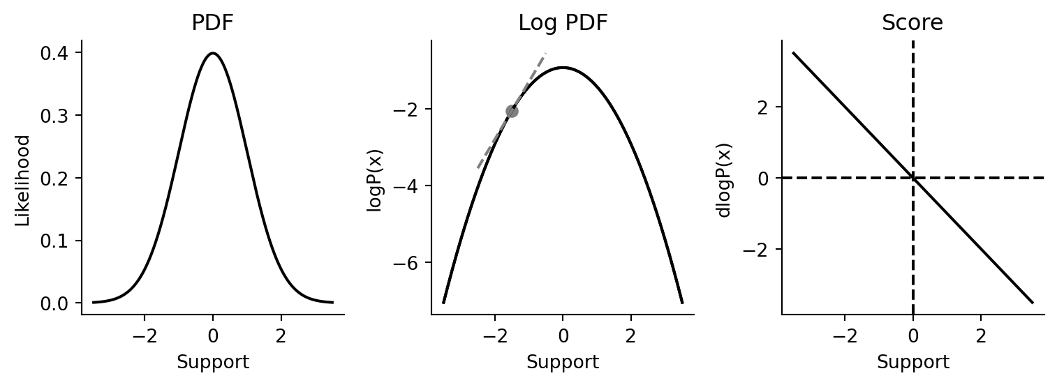
The same chapter provides a formal proof of this final, crucial connection.
Read the section Maximum Likelihood Estimation, focusing on Theorem 26.4 (MLE Minimizes KL Divergence). Follow the proof that starts with the definition of KL divergence and shows its equivalence to the negative log-likelihood. The summary table at the end of the section provides a perfect conceptual recap.
To reinforce this key idea, the following video offers a concise, practical explanation.
What is the difference between negative log likelihood and cross entropy? (in neural networks)
This video directly tackles the question of the relationship between Negative Log Likelihood and Cross-Entropy in the context of neural networks.
First, watch the derivation of the Negative Log Likelihood loss for a classification model. Then, watch as the formal definition of cross-entropy is introduced and shown to be mathematically identical to the NLL expression you just saw.
5. Practical Implications for Model Training
This theoretical foundation has direct, practical consequences for engineering robust AI systems.
Why Cross-Entropy is Superior to MSE for Classification
The primary reason is its effect on gradients during backpropagation. When you combine a softmax output with a cross-entropy loss, the gradient of the loss with respect to the pre-softmax activations (the logits, ) has a beautifully simple form:
where is the predicted probability and is the true label (0 or 1). The gradient is simply the error in the prediction. When the model is confidently wrong (e.g., is near 0 but is 1), the gradient is large, providing a strong learning signal.
In contrast, the gradient for MSE loss with a sigmoid/softmax output contains a term. This derivative term approaches zero when the activation saturates (i.e., when the output is near 0 or 1). This means if the model is confidently wrong, the gradients vanish, and learning stalls. Cross-entropy's probabilistic formulation elegantly sidesteps this critical problem.
This is one of the most important practical insights in training classifiers.
Read the section Cross-Entropy Loss for Classification. Focus on the subsection Why Cross-Entropy Beats MSE. The mathematical derivations and the final plot comparing the gradient magnitudes provide a definitive, evidence-based reason for this standard practice.
The Asymmetry of KL Divergence
A final, advanced point is that KL divergence is not a true "distance" metric because it is asymmetric: . The direction matters.
- Forward KL , used in MLE, is "mean-seeking." It tries to ensure that where has probability mass, also has probability mass. It leads to inclusive, broader approximations.
- Reverse KL is "mode-seeking." It tries to ensure that where has high probability mass, also does. It punishes for putting mass in places where has none, leading to exclusive, sharper approximations that focus on a single mode.
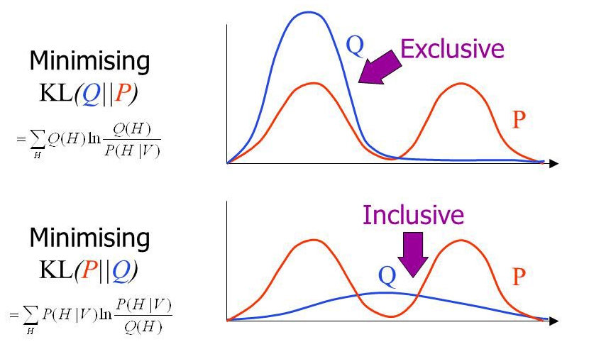
While standard classification uses the forward KL implicitly through MLE, understanding this distinction is crucial for more advanced generative models like Variational Autoencoders (VAEs), which often use the reverse form.
Conclusion
In this lesson, you have completed your mathematical toolkit by connecting the worlds of probability, information theory, and machine learning. You've moved beyond simply using loss functions to understanding their fundamental justification.
Key takeaways from this lesson include:
- Common loss functions are not arbitrary; they are derived from the principle of Maximum Likelihood Estimation (MLE).
- Minimizing the Negative Log-Likelihood (NLL) is the operational way to perform MLE. For regression with a Gaussian noise assumption, this yields Mean Squared Error.
- For classification, training a model is equivalent to minimizing the KL Divergence between the data distribution and the model's predicted distribution.
- Minimizing KL Divergence is, in turn, equivalent to minimizing the Cross-Entropy loss.
- This establishes the core equivalence: MLE KL Divergence Minimization Cross-Entropy Minimization.
- This probabilistic view explains why Cross-Entropy provides more stable gradients than MSE for classification tasks, preventing the saturation problem.
Having established the what (calculus), the how (linear algebra), and the why (probability), we are now ready to explore how modern frameworks put this all together. In the next lesson, we will investigate the mechanics of automatic differentiation and the structure of dynamic computational graphs, revealing the magic that powers frameworks like PyTorch and enables the efficient computation of the gradients we've discussed.