In our previous lessons, we built a robust mathematical toolkit, covering the calculus of backpropagation, the linear algebra of model structure, and the probabilistic justification for our loss functions. You now understand what we're optimizing and why we're optimizing it. This lesson bridges the gap to the how: the engine that actually computes the gradients for our complex models. Your goal is to move beyond simply calling .backward(), and this lesson will pull back the curtain on that exact mechanism.
We will explore automatic differentiation (AD), the foundational technology of all modern deep learning frameworks. You will learn how AD differs from numerical and symbolic differentiation, and why it's uniquely suited for deep learning. We will dissect its two primary modes—forward and reverse—and understand their efficiency trade-offs. Most importantly, you will see how these concepts are realized in PyTorch through dynamic computational graphs, setting the stage for you to build custom, high-performance components.
1. The Challenge of Differentiation in Deep Learning
To train a model, we need to compute the gradient of a scalar loss function with respect to potentially millions of parameters (). How can we do this efficiently and accurately? There are three main approaches.
First, Numerical Differentiation uses the definition of a derivative to approximate it with finite differences, like . While simple to implement, it's computationally expensive (requiring multiple forward passes per parameter) and numerically unstable. Its primary role in modern engineering is not for training, but for verifying the correctness of more complex gradient implementations—a technique called gradient checking.
Second, Symbolic Differentiation, the method you learned in calculus class, applies derivative rules (product rule, chain rule, etc.) to a mathematical expression to derive a new expression for the gradient. While exact, this method suffers from "expression swell": the symbolic representation of the gradient for a deep neural network can become astronomically large and inefficient to evaluate.
This leaves us with the third and most effective method: Automatic Differentiation (AD).
Lecture 4 - Automatic Differentiation
This lecture from the Deep Learning Systems course at CMU provides an excellent overview of the problem and the different methods for computing gradients.
First, watch the recap of why we need gradients for optimization at the beginning. Then, focus on the explanations of Numerical Differentiation, noting its main use for gradient checking, and Symbolic Differentiation, understanding its problem with expression swell and redundant computation.
2. Computational Graphs: The Language of AD
Automatic differentiation operates on a computational graph. This is a directed acyclic graph (DAG) where nodes represent either variables (tensors) or operations (e.g., +, *, log, sin), and edges represent the flow of data. Every function, no matter how complex, can be decomposed into a sequence of elementary operations on a graph.
A critical distinction in deep learning frameworks is between static and dynamic computational graphs.
- Static Graphs (e.g., TensorFlow 1.x): You first define the entire graph structure. You then compile this graph and execute it by feeding data into it. This allows for significant upfront optimization but is rigid and less intuitive to debug.
- Dynamic Graphs (e.g., PyTorch, modern TensorFlow): The graph is built on-the-fly as the forward pass code is executed. This "define-by-run" approach is more flexible, more "Pythonic," and allows for the use of standard Python control flow (
ifstatements,forloops) within your model.
PyTorch's autograd engine is built entirely on the principle of dynamic graphs.
Lecture 4 - Automatic Differentiation
The same lecture introduces the concept of a computational graph and walks through an evaluation.
Watch the section on computational graphs. Pay attention to how a mathematical expression is translated into a graph and how values are propagated forward through it.
[PDF] Automatic differentiation in PyTorch - OpenReview
This paper, presented at NeurIPS, details the design choices behind PyTorch's autograd. It directly contrasts PyTorch's approach with static graph frameworks.
Read the introduction in Section 1. Focus on the two distinguishing features: dynamic execution and eager execution. This text explains the core philosophy that makes PyTorch's approach so powerful and user-friendly.
3. The Two Modes of Automatic Differentiation
AD works by applying the chain rule to the elementary operations in the computational graph. It does this in one of two ways: forward mode or reverse mode.
Forward Mode AD
In forward mode, we traverse the graph from inputs to outputs. At each node, we compute both the value of that node (the primal) and the derivative of that node with respect to one input variable (the tangent). You can think of it as propagating (value, derivative) pairs forward through the graph.
- Efficiency: One forward pass computes the derivatives of all outputs with respect to one input. To get the full gradient of a scalar loss with respect to parameters, you would need to perform forward passes.
- When to use: It is efficient when the number of inputs is much smaller than the number of outputs ().
Reverse Mode AD (Backpropagation)
In reverse mode, we first perform a full forward pass, computing the value of each node and caching any intermediate results needed for gradients. Then, we traverse the graph in reverse, from the final output back to the inputs. At each node, we compute the derivative of the final output with respect to that node's value (the adjoint). This is the essence of backpropagation.
- Efficiency: One forward pass followed by one backward pass computes the derivatives of one output with respect to all inputs.
- When to use: It is efficient when the number of inputs is much larger than the number of outputs ().
For training neural networks, we have a single scalar loss output () and millions of parameters as inputs ( is huge). Therefore, reverse mode AD is the fundamental algorithm that makes modern deep learning computationally feasible.

Lecture 4 - Automatic Differentiation
The CMU lecture provides a detailed, step-by-step derivation of both modes on the same computational graph, making the comparison very clear.
First, watch the walkthrough of Forward Mode AD. Follow the propagation of the v_dot terms. Then, watch the detailed derivation of Reverse Mode AD, focusing on how the adjoint values are computed backward. Finally, pay close attention to the explanation of handling multiple pathways, as this is crucial for understanding how gradients from different parts of a network are accumulated.
To solidify your understanding, the following text provides a more formal definition of the terms used in each mode.
What's Automatic Differentiation?
This Hugging Face blog post gives a clear, text-based explanation of the mechanics and terminology of AD.
First, read the main section on Automatic Differentiation to understand the concepts of an evaluation trace and computational graph. Then, read the sections on Forward Mode AD, focusing on the definition of tangents and the conclusion about its inefficiency for neural networks. Finally, read the section on Reverse Mode AD, understanding the concept of adjoints and why it is optimal when n \gg m.
4. Reverse Mode AD in PyTorch: autograd
PyTorch's autograd engine is a sophisticated implementation of reverse-mode AD on a dynamic computational graph. When you perform an operation on tensors where requires_grad=True, PyTorch builds up this graph.
Each tensor has several key attributes:
data: The underlying data of the tensor.requires_grad: A boolean. IfTrue, operations on this tensor are tracked.grad: Stores the value of the gradient after.backward()is called. It isNoneby default and is only populated for leaf tensors withrequires_grad=True.grad_fn: This is the backward link in the graph. It references the function that created the tensor (e.g.,MulBackward,AddBackward). Leaf tensors (created by the user) have agrad_fnofNone.is_leaf:Trueif the tensor was created by the user (e.g.,torch.tensor(...)or annn.Parameter).Falseif it's the result of an operation.
When you call loss.backward(), PyTorch traverses this graph backward from the loss tensor, using the grad_fn at each step to calculate and pass gradients to the next node, until it reaches the leaf nodes (your model parameters). The gradients are then accumulated in the .grad attribute of these leaf tensors.
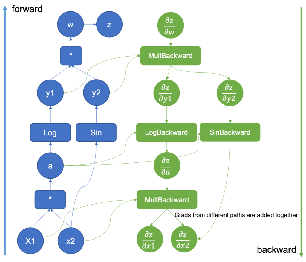
PyTorch Autograd Explained - In-depth Tutorial
This tutorial provides a fantastic visual explanation of how PyTorch's autograd works internally, connecting the theory to the actual objects and attributes.
Watch the initial explanation of tensor attributes (grad_fn, is_leaf, etc.). Then, see how a simple backward graph is created. The next section visualizes a more complex graph, showing how gradients converge and are accumulated at leaf nodes. Finally, watch the segment on in-place operations and versioning, as this is a critical detail for writing safe and correct PyTorch code.
For a deeper dive into the engineering, the PyTorch paper explains how the core logic is implemented.
[PDF] Automatic differentiation in PyTorch - OpenReview
This paper provides the "under-the-hood" view you're looking for, explaining the C++ core and how tricky edge cases are handled.
Read Section 3, Implementation, to understand the internal representation. Note how a Variable (now just Tensor) holds a reference to a graph of Function objects, and that the core logic is in C++ for performance. Then, read Section 3.1, Supporting in-place operations, to learn how PyTorch detects potentially correctness-breaking operations using version counters. This is a key piece of engineering that ensures the integrity of the backward pass.
Conclusion
In this lesson, you've unpacked the "magic" behind deep learning optimization. You've gone from a high-level understanding of gradients to the specific mechanics of how they are computed in a modern framework like PyTorch.
The key takeaways are:
- Automatic Differentiation (AD) is the engine of deep learning, offering a precise and efficient way to compute gradients by applying the chain rule to a sequence of elementary operations.
- Computations are represented by Computational Graphs. PyTorch uses dynamic, define-by-run graphs, which are flexible and integrate seamlessly with Python.
- Forward Mode AD computes derivatives with respect to one input at a time and is inefficient for training, which involves many inputs (parameters).
- Reverse Mode AD (Backpropagation) is the workhorse of deep learning. It computes derivatives with respect to all inputs at once, making it highly efficient for the many-to-one mapping of parameters to a scalar loss.
- PyTorch's
autogradsystem implements reverse mode AD usinggrad_fnattributes on tensors to build the backward graph dynamically.
You now understand the theoretical and practical machinery that executes backpropagation. This knowledge is not just academic; it is the foundation for debugging complex models, optimizing performance, and creating novel neural network components.
In the next lesson, we will put this knowledge into practice. You will implement a custom PyTorch Autograd function, where you will manually define the forward and backward passes for a non-standard operation. This will solidify your understanding and give you the power to extend PyTorch beyond its built-in library.