Multivariate Chain Rule and Backpropagation

Welcome to the first lesson in your journey to mastering the foundations of AI. Our goal in this initial module is to build the essential mathematical toolkit you'll need to understand and design complex neural networks from first principles. This lesson tackles a cornerstone concept that separates API consumers from system architects: backpropagation.

You've expressed a desire to move beyond black boxes and understand the underlying mathematics. This lesson is designed to do exactly that. We will derive the backpropagation algorithm from its roots in multivariable calculus, focusing on the chain rule as it applies to functions with vector inputs. By the end of our 60 minutes, you will not only understand what backpropagation does but why it is a direct and efficient application of the chain rule. This will set a strong foundation for the entire curriculum.

1. The Need for a Systematic Approach: Computational Graphs

When we train a neural network, our goal is to adjust its weights to minimize a loss function. This is an optimization problem solved with gradient descent, which requires us to compute the gradient of the scalar loss with respect to every weight in the network.

For a simple linear model, one might be tempted to write out the full loss function and derive the gradients manually. However, as models become deep, with millions of parameters and complex interdependencies, this approach quickly becomes intractable.

Lecture 6: Backpropagation

To understand why manual derivations don't scale, watch this segment from the "Lecture 6: Backpropagation" video by Michigan Online. It introduces the core problems with manual derivation and presents the computational graph as the data structure that enables a modular and scalable solution.

Watch from the beginning of the discussion on strategy one, which covers the shortcomings of manual derivation. Then, continue from the introduction of computational graphs to see how they represent complex computations in a structured way.

As the video explains, a computational graph breaks down a complex function into a sequence of simple, elementary operations (nodes). This modularity is key. To compute the overall gradient, we only need to know how to compute gradients for these simple operations and how to combine them. The algorithm that traverses this graph backward to compute gradients is backpropagation.

2. Backpropagation Intuition: The Chain Rule on a Scalar Graph

At its heart, backpropagation is nothing more than a recursive application of the chain rule from calculus. Let's build our intuition with a simple scalar example before moving to vectors.

Imagine the function $f (x, y, z) = (x + y) \cdot z$ . We can represent this as a computational graph where an addition node feeds into a multiplication node. The backward pass calculates the gradient of the final output, $f$ , with respect to each input, $x$ , $y$ , and $z$ .

This process introduces three key terms:

Upstream Gradient: The gradient of the final loss flowing into a node from later in the graph.
Local Gradient: The gradient of a node's output with respect to its immediate inputs.
Downstream Gradient: The gradient of the final loss with respect to a node's inputs, calculated by combining the upstream and local gradients. This is what gets passed backward to the preceding nodes.

The chain rule tells us how to combine these:

Downstream Gradient = Upstream Gradient \times Local Gradient

Stanford CS231N | Spring 2025 | Lecture 4: Neural Networks and Backpropagation

This video from Stanford Online provides an excellent, step-by-step walkthrough of backpropagation on the scalar function we just discussed. It clearly visualizes the forward pass (computing the values) and the backward pass (propagating the gradients).

Watch the segment from back propagation. Pay close attention to how the presenter calculates the local gradients for the addition and multiplication gates, and then uses the chain rule to compute the downstream gradients for x, y, and z.

This scalar example reveals the core mechanic: backpropagation is an algorithm that starts at the end of the graph (with an initial upstream gradient of 1) and recursively applies the chain rule at each node to compute the gradients with respect to all inputs.

3. Generalizing to Vectors: The Jacobian Matrix

In real neural networks, our operations are not on scalars but on vectors, matrices, and tensors. To apply the chain rule here, we need to generalize the concept of a derivative.

For a function $f : R^{n} \to R^{m}$ that takes a vector of size $n$ and produces a vector of size $m$ , the derivative is no longer a single number. It becomes a matrix of all possible partial derivatives, known as the Jacobian matrix.

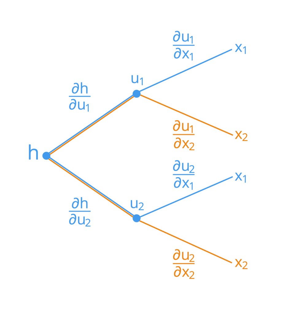
This graph illustrates the multivariate chain rule. The final output `h` depends on intermediate variables `u1` and `u2`, which in turn depend on inputs `x1` and `x2`. The gradient of `h` with respect to `x1` must account for both paths through `u1` and `u2`.

Derivatives, Backpropagation, and Vectorization

The CS231n course notes from Stanford provide a concise and formal definition of the Jacobian and the multivariate chain rule. This will provide the mathematical rigor needed to understand backpropagation in its true form.

First, read the section Gradient: Vector in, scalar out to solidify your understanding of the gradient. Next, focus on the section Jacobian: Vector in, Vector out. This defines the Jacobian matrix \frac{\partial\mathbf{y}}{\partial\mathbf{x}} for a vector-to-vector function. Notice its dimensions are M \times N. Finally, read the crucial part on the vector chain rule. The key takeaway is that the scalar chain rule's multiplication becomes a matrix multiplication of Jacobians: \frac{\partial\mathbf{z}}{\partial\mathbf{x}} = \frac{\partial\mathbf{z}}{\partial\mathbf{y}} \frac{\partial\mathbf{y}}{\partial\mathbf{x}}.

Pay close attention to the dimensions. If $y = f (x)$ and $z = g (y)$ , with $x \in R^{N}, y \in R^{M}, z \in R^{K}$ , then:

$\frac{\partial y}{\partial x}$ is an $M \times N$ Jacobian.
$\frac{\partial z}{\partial y}$ is a $K \times M$ Jacobian.
Their product, $\frac{\partial z}{\partial x}$ , is a $K \times N$ Jacobian, as expected.

4. Deriving Backpropagation for a Neural Network

We now have all the components to formally derive backpropagation. Let's consider a $k$ -layered neural network. The forward pass computes a sequence of activations:

a^{(l)} = σ (z^{(l)}) where z^{(l)} = W^{(l)} a^{(l - 1)} + b^{(l)}

The final output is a scalar loss, $L = c_{y} (a^{(k)})$ . Our goal is to compute the gradients $\frac{\partial L}{\partial W ^{(l)}}$ and $\frac{\partial L}{\partial b ^{(l)}}$ for all layers $l$ .

Let's define the "error" signal $δ^{(l)}$ as the gradient of the loss with respect to the pre-activation vector $z^{(l)}$ :

δ^{(l)} := \frac{\partial L}{\partial z ^{(l)}}

This $δ^{(l)}$ is our upstream gradient flowing into layer $l$ . Using the chain rule, we can derive a recursive formula for it.

This diagram shows the core backpropagation equations for a single layer $ (L) $. The gradient of the cost $ C $ with respect to the weights $ w_{jk}^{(L-1)} $ and the previous layer's activations $ a_k^{(L-1)} $ are derived using the chain rule, propagating the gradient $ \frac{\partial C}{\partial a_j^{(L)}} $ backward through the activation $ a_j^{(L)} $ and the pre-activation $ z_j^{(L)} $.

The following paper provides a formal, matrix-based proof of the backpropagation algorithm. We will focus on its statement of the algorithm and the intuition behind its proof.

[PDF] An induction proof of the backpropagation algorithm in matrix notation

This paper rigorously defines the backpropagation algorithm using matrix calculus. This is the kind of "under the hood" derivation you're looking for.

First, read Theorem 1 (Backpropagation algorithm) in Section 4. This presents the core recursive equations: Equation (23): \delta^l = ((W^{l+1}_{\bullet})^T \cdot \delta^{l+1}) \circ \tilde{\Sigma}^l(z^l) This shows how to compute the error \delta^l for the current layer using the error \delta^{l+1} from the next layer. This is the chain rule in action, propagating the gradient backward through the weight matrix W^{l+1} and the activation function derivative \tilde{\Sigma}^l. Equation (24): \nabla_{W^l}c_{xy} = \text{vec}(\delta^l \cdot (\Sigma^{l-1}(z^{l-1})^T \ 1)) This shows how to compute the gradient for the weights W^l once you have the error \delta^l. It's the product of the error and the activations from the previous layer. Next, to see how these are derived, skim the Base case subsection in Section 5.1, particularly the derivation for \nabla_{W^3}c_{xy} and \nabla_{W^2}c_{xy}. You don't need to follow every single algebraic step, but observe the repeated application of the chain rule (Theorem 5 in their appendix) to peel back one layer at a time. This is the explicit mathematical machinery of backpropagation.

The Efficiency of Jacobian-Vector Products

A crucial insight, both for theory and for practical implementation, is that we never explicitly form the massive Jacobian matrices. The derivations in the paper and the formulas in Theorem 1 are actually clever ways of expressing a Jacobian-vector product (JVP).

The term $((W_{∙}^{l + 1})^{T} \cdot δ^{l + 1})$ is not just an arbitrary matrix multiplication; it is the efficient implementation of multiplying the upstream gradient vector $δ^{l + 1}$ by the transposed Jacobian of the linear transformation $z^{(l + 1)} = W^{(l + 1)} a^{(l)}$ .

Lecture 6: Backpropagation

This final video segment explains this critical concept of implicit Jacobian-vector products and summarizes backpropagation as "reverse-mode automatic differentiation."

Watch the section on vector-valued functions to see how the scalar chain rule extends to Jacobians and vectors. Then, watch the detailed example of matrix multiplication. This is a masterclass in how to derive the backward pass for an operation without ever forming the Jacobian. The logic of reasoning about one element at a time to uncover a general matrix expression is a powerful technique. Finally, watch the summary view of backpropagation as a chain of Jacobians. This frames backpropagation as an efficient right-to-left evaluation of the chain rule, where you are always performing matrix-vector products, which is far more efficient than the matrix-matrix products you would get with a left-to-right evaluation ("forward-mode differentiation").

This "right-to-left" evaluation, or reverse-mode automatic differentiation, is precisely what makes backpropagation efficient for typical deep learning scenarios where we have many inputs (weights) and a single scalar output (loss).

Conclusion

In this lesson, we have deconstructed backpropagation and revealed its mathematical core. You should now be able to explain how it is a direct and computationally efficient application of the multivariate chain rule.

Here are the key takeaways:

Computational Graphs provide a modular structure for representing complex functions, which is essential for systematic gradient computation.
Backpropagation is an algorithm that traverses this graph in reverse, applying the chain rule at each node to compute the gradient of a final scalar output with respect to all preceding variables.
For functions with vector inputs and outputs, the derivative is the Jacobian matrix, and the chain rule involves matrix multiplication of Jacobians.
The core computation in backpropagation is a Jacobian-vector product, which is almost always computed implicitly via efficient expressions (like simple matrix multiplies) rather than by explicitly forming the enormous and sparse Jacobian matrix.

You have now established the fundamental calculus-based mechanism for training neural networks. In our next lesson, we will shift our focus to linear algebra and explore eigenvalues, eigenvectors, and Singular Value Decomposition (SVD). These concepts are not just abstract tools; they are critical for analyzing model properties, understanding data transformations, and are the foundation for powerful techniques like low-rank approximation, which you'll encounter in modern model optimization.

Recommended resources