Data Dependencies and Parallelization

1. The Fundamental Condition for Parallelism

At its core, the ability to parallelize two statements, let's call them S1 and S2, hinges on a simple question: does the order of their execution matter?

If the result of running S1; S2; is identical to running S2; S1;, then they are independent and can be executed in parallel. If the order does matter, a data dependency exists between them, which acts as a constraint.

Consider these simple C++ assignments:

// Block 1: Independent Statements
int a = 10; // S1
int b = 20; // S2

Here, swapping the order of S1 and S2 has no effect on the final state of the program. They can run in parallel.

// Block 2: Dependent Statements
int a = 10;   // S1
int b = a + 5; // S2

In this case, S2 needs the value of a computed by S1. Executing S2 before S1 would produce an incorrect (or undefined) result. This is a data dependency. Any relationship that enforces a specific execution order is a dependency. Let's formalize the different types.

2. The Three Types of Data Dependencies

There are three primary types of data dependencies that can occur between two statements, S1 followed by S2. These are often explained using low-level instructions, as dependencies are fundamentally about how memory or registers are accessed.

To get a clear and concise overview of these dependencies, let's watch a short video from Georgia Tech's High Performance Computer Architecture course.

Let's summarize and contextualize what you just saw with C++ examples.

a. True Dependence (Read-After-Write / RAW)

• Definition: S2 reads a variable that S1 writes.
• Alternative Name: Flow Dependence. This is the most intuitive type of dependency—the result of S1 "flows" to S2.
• Example:

  // S1: Write to 'x'
  x = calculate_value();
  // S2: Read from 'x'
  y = x * 2;
  

• Constraint: This is a fundamental and unbreakable dependency. S2 cannot begin until S1 has completed.

b. Anti-Dependence (Write-After-Read / WAR)

• Definition: S2 writes to a variable that S1 reads.
• Example:

  // S1: Read from 'x'
  y = x * 2;
  // S2: Write to 'x'
  x = 100;
  

• Constraint: If S2 were to execute before S1, S1 would incorrectly use the new value of x (100) instead of its original value. The original execution order must be preserved.

c. Output Dependence (Write-After-Write / WAW)

• Definition: S2 writes to the same variable that S1 also writes.
• Example:

  // S1: Write to 'x'
  x = 10;
  // S2: Write to 'x'
  x = 20;
  

• Constraint: If S2 executed before S1, the final value of x would be 10 instead of the correct 20. The order of writes must be maintained.

"False" vs. "True" Dependencies

As the video mentioned, WAR and WAW dependencies are often called false or name dependencies. This is because the dependency exists due to the re-use of a variable name (or memory location), not because of a true flow of data. These can often be eliminated by renaming variables.

For instance, the WAR example could be rewritten to remove the dependency:

// Original (WAR dependency)
y = x * 2;
x = 100;

// Rewritten (no dependency)
y = x * 2;
int x_new = 100; // Use a new variable

This kind of transformation is a common optimization performed by both compilers and parallel programmers. RAW dependencies, however, are fundamental to the algorithm's logic and cannot be removed so easily.

3. A Systematic Approach to Finding Dependencies

Manually inspecting code for dependencies can be error-prone. A more structured method is to analyze the read set (variables an instruction reads) and write set (variables an instruction writes) for each statement.

To summarize the method shown in the video for two statements, S1 followed by S2:

1. Identify Read and Write Sets:

   • ReadSet(S): The set of variables read by statement S.
   • WriteSet(S): The set of variables written by statement S.

2. Check for Intersections:

   • RAW: WriteSet(S1) intersects with ReadSet(S2).
   • WAR: ReadSet(S1) intersects with WriteSet(S2).
   • WAW: WriteSet(S1) intersects with WriteSet(S2).

4. Practice Exercise

Let's apply this systematic approach. The following image shows a sequence of four instructions. Your task is to identify all the RAW, WAR, and WAW dependencies between them.

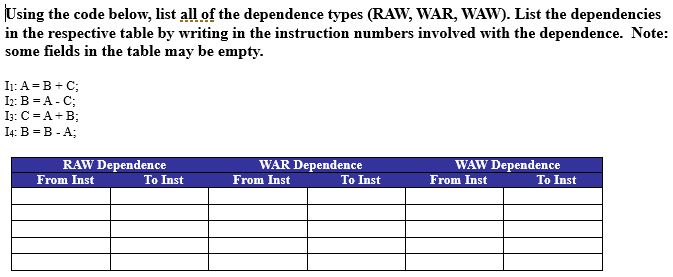
Take a moment to analyze the instructions using the read/write set method, and determine which instruction pairs have which dependencies.

Solution

First, let's list the read and write sets for each instruction:

• I1: R3 = R1 + R2
  • ReadSet(I1) = {R1, R2}
  • WriteSet(I1) = {R3}
• I2: R5 = R3 + R4
  • ReadSet(I2) = {R3, R4}
  • WriteSet(I2) = {R5}
• I3: R3 = R5 + R4
  • ReadSet(I3) = {R5, R4}
  • WriteSet(I3) = {R3}
• I4: R6 = R3 + R2
  • ReadSet(I4) = {R3, R2}
  • WriteSet(I4) = {R6}

Now, let's check for dependencies:

• RAW (Read-After-Write):

  • I1 -> I2: WriteSet(I1)={R3}, ReadSet(I2)={R3, R4}. Intersection on R3.
  • I2 -> I3: WriteSet(I2)={R5}, ReadSet(I3)={R5, R4}. Intersection on R5.
  • I3 -> I4: WriteSet(I3)={R3}, ReadSet(I4)={R3, R2}. Intersection on R3.

• WAR (Write-After-Read):

  • I2 -> I3: ReadSet(I2)={R3, R4}, WriteSet(I3)={R3}. Intersection on R3. (I2 must read the old R3 before I3 overwrites it).

• WAW (Write-After-Write):

  • I1 -> I3: WriteSet(I1)={R3}, WriteSet(I3)={R3}. Intersection on R3. (I1 writes to R3, and later I3 also writes to R3).

5. Dependencies in Loops

In practice, most opportunities for significant parallelism are found within loops. Identifying dependencies in loops is crucial, especially a type known as a loop-carried dependence.

As you read, the key distinction is:

• Loop-independent dependence: The dependency exists within a single iteration of the loop. The iterations themselves are independent of each other and can be parallelized.

  for (int i = 0; i < N; ++i) {
      float temp = a[i] * 2.0f; // S1
      b[i] = temp + 1.0f;      // S2 (RAW on 'temp')
  }
  

  Each iteration i can be executed independently of iteration i+1.

• Loop-carried dependence: The dependency is between different iterations. This is the primary obstacle to parallelizing loops.

  for (int i = 1; i < N; ++i) {
      // Reads a value from the PREVIOUS iteration.
      a[i] = a[i-1] + 5;
  }
  

  Here, iteration i has a RAW dependency on iteration i-1. You cannot calculate a[2] until a[1] is finished, making parallel execution of the iterations impossible without transforming the algorithm.

Finally, be aware of hidden dependencies, such as calls to functions with side effects (e.g., modifying a global variable) or I/O operations (printf), which implicitly write to a shared resource (the output stream).

Conclusion

In this lesson, you've learned to identify the fundamental constraints that govern parallelism. This skill is non-negotiable for anyone looking to write correct and efficient parallel code.

Key Takeaways:

• Three types of data dependencies constrain parallel execution: Read-After-Write (RAW), Write-After-Read (WAR), and Write-After-Write (WAW).
• RAW dependencies are "true" dependencies representing a flow of data, while WAR and WAW are "name" dependencies caused by variable reuse and can sometimes be eliminated.
• A systematic way to find dependencies is to define the read set and write set for each statement and check for intersections between statement pairs.
• Loop-carried dependencies, where one loop iteration depends on the result of a previous one, are the main reason loops cannot be naively parallelized.

Preview of the Next Lesson

Now that we know how to identify the parts of a program that cannot be parallelized, a natural next question is: "If only part of my program can be parallel, how much faster can my whole program get?" In the next lesson, we will introduce Amdahl's Law, a classic formula used to calculate the theoretical maximum speedup of a parallel algorithm.