Amdahl's Law for Parallel Speedup

1. The Concept of Speedup and Its Ideal Limit

Before we dive into Amdahl's Law, let's formally define what we mean by "speedup."

Speedup, denoted as $S(P)$, is the ratio of the execution time of a program on a single processor to its execution time on $P$ parallel processors.

Where:

• $T_1$ is the execution time on one processor.
• $T_P$ is the execution time on $P$ processors.

In an ideal world, if you use $P$ processors, your program would run $P$ times faster, meaning $S(P)=P$. This is known as linear speedup. For example, with 8 processors, you'd hope for an 8x speedup. However, as our last lesson on data dependencies showed, some parts of the program are sequential and cannot be divided among processors. This serial fraction prevents us from achieving perfect linear speedup.

2. Deriving Amdahl's Law

Gene Amdahl formalized this relationship in 1967. His insight was to model the total execution time as a combination of two distinct parts: a fraction that is perfectly sequential and a fraction that is perfectly parallelizable.

To see how this works and how the famous formula is derived, let's watch a short video that explains it from first principles.

Let's quickly recap the derivation, solidifying the terms:

1. Let $s$ be the fraction of the program's execution time that is serial (cannot be parallelized).

2. Let $f$ (or $p$ in some texts) be the fraction that is parallelizable.

3. By definition, $s+f=1$.

4. The total time on a single processor, $T_1$, can be normalized to 1 unit of time. So, $T_1=s+f=1$.

5. When running on $P$ processors:

   • The serial part still takes time $s$.
   • The parallelizable part can, ideally, be sped up by a factor of $P$, so it takes time $f/P$.

6. The total time on $P$ processors is therefore $T_P=s+\frac{f}{P}$.

7. The speedup, $S(P)=\frac{T_1}{T_P}$, becomes:

   $$S(P)=\frac{1}{s+\frac{f}{P}}=\frac{1}{s+\frac{1-s}{P}}$$

This final equation is Amdahl's Law.

3. The Dominance of the Serial Fraction

The most profound implication of Amdahl's Law becomes clear when we consider what happens as we add a very large number of processors. What is the limit of speedup as $P\to \infty$?

As $P$ becomes very large, the term $\frac{1-s}{P}$ approaches zero.

This is the central message of Amdahl's Law: the theoretical maximum speedup is determined entirely by the serial fraction of the code.

• If 50% of your code is serial ($s=0.5$), the maximum speedup you can ever achieve is $1/0.5=2x$, even with a million processors.
• If 10% of your code is serial ($s=0.1$), the maximum speedup is $1/0.1=10x$.
• If only 1% of your code is serial ($s=0.01$), the maximum speedup is $1/0.01=100x$.

The following graph visualizes this limitation powerfully.

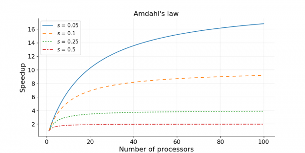
Notice how quickly the speedup curves flatten out, especially for higher values of the serial fraction $s$. Adding more processors yields diminishing returns, and the bottleneck created by the serial part comes to dominate performance.

4. Applying the Formula: Worked Examples

Let's put the formula to work with a couple of practical calculations. The following video walks through several examples of plugging numbers into the formula.

Now, it's your turn to apply the law.

Practice Problem:

Imagine you are working on a simulation program. A profiler tells you that 95% of the runtime is spent in a large, parallelizable loop, while the remaining 5% is for initial setup and final report generation (which are serial).

1. What is the expected speedup on a modern 16-core workstation?
2. Your company is considering buying a supercomputer with 1024 cores. What is the theoretical speedup you could get on that machine?
3. What is the absolute maximum speedup you could ever hope to achieve for this program, regardless of the number of cores?

Take a moment to calculate the answers.

Solution:

Here, the serial fraction is $s=0.05$, and the parallelizable fraction is $f=0.95$.

1. On 16 cores ($P=16$):

   $$S(16)=\frac{1}{0.05+\frac{0.95}{16}}=\frac{1}{0.05+0.059375}=\frac{1}{0.109375}\approx 9.14x$$

   Even with 95% parallel code, you get just over 9x speedup on 16 cores, not 16x.

2. On 1024 cores ($P=1024$):

   $$S(1024)=\frac{1}{0.05+\frac{0.95}{1024}}=\frac{1}{0.05+0.000927}=\frac{1}{0.050927}\approx 19.64x$$

   Notice the sharply diminishing returns. Increasing the core count by 64x (from 16 to 1024) only doubles the speedup.

3. Maximum Theoretical Speedup:

   $$S_{max}=\frac{1}{s}=\frac{1}{0.05}=20x$$

   No matter how many processors you use, you can never make this program run more than 20 times faster than the original.

5. Assumptions and Limitations

Amdahl's Law is a powerful tool for developing intuition, but it's important to recognize its underlying assumption. It analyzes strong scaling, where the problem size is fixed. You are using more processors to solve the same problem, faster.

The law also makes simplifying assumptions, ignoring real-world complexities such as:

• Communication overhead: Processors need to coordinate, which takes time.
• Memory bandwidth limitations: All cores competing for access to RAM can create a new bottleneck.
• Load balancing issues: It might not be possible to divide the work perfectly evenly.

Despite these simplifications, Amdahl's Law provides an essential, if optimistic, upper bound on the performance you can expect.

Conclusion

In this lesson, we dissected one of the most fundamental principles of parallel computing. The insights you've gained are critical for setting realistic performance expectations and for identifying where to focus optimization efforts.

Key Takeaways:

• Amdahl's Law provides the theoretical speedup of a program based on its serial fraction ($s$) and the number of processors ($P$): $S(P)=1/(s+(1-s)/P)$.
• The performance gain from parallelization is ultimately limited by the serial portion of the code.
• The absolute maximum speedup an application can achieve is $1/s$, regardless of how many processors are used.
• Amdahl's Law describes strong scaling, where the goal is to solve a fixed-size problem faster.

Preview of the Next Lesson

Amdahl's Law can seem pessimistic. It suggests that adding more processors offers limited benefits. But what if, instead of solving the same problem faster, we used more processors to solve a bigger or more detailed problem in the same amount of time? This perspective, known as weak scaling, is described by Gustafson's Law, and it will be the subject of our next lesson.