Loss Functions and Gradient Descent

What is a Loss Function?

In the previous lesson, we used metrics like the F1-score to evaluate our model from a business or application perspective. However, for a model to learn algorithmically, it needs a different kind of signal. It needs a loss function (or error function).

A loss function's job is to calculate a single number that represents how "wrong" a model's predictions are compared to the actual target values. The higher the number, the worse the model is doing. The goal of training is to adjust the model's internal parameters—its weights and biases—to make this loss as small as possible.

It's useful to distinguish between a loss function and a cost function. While often used interchangeably, a loss function typically calculates the error for a single training example, while a cost function is the average of the loss over the entire training dataset.

While there are many types of loss functions, they are generally chosen based on the task (e.g., regression or classification). Two of the most common are:

• Mean Squared Error (MSE): Used for regression tasks, like predicting a house price. It calculates the average of the squared differences between the predicted and actual values. Squaring the error penalizes larger mistakes more heavily.
• Cross-Entropy Loss: Used for classification tasks. It measures how different the model's predicted probabilities are from the true class labels (0s and 1s).

The key takeaway is that the loss function provides the objective that the training process aims to minimize. But how does it do that?

How Models Learn: The Intuition of Gradient Descent

Once we have a loss function, we can think of it as a landscape where the "low ground" or valleys represent a small loss and the "high ground" or hills represent a large loss. Our model's parameters (its weights) determine our position on this landscape. Our goal is to find the lowest point in this landscape.

The algorithm used to do this is called gradient descent. Imagine you are standing on a foggy hillside and want to get to the bottom. You can't see the valley, but you can feel the slope of the ground beneath your feet. The most straightforward strategy is to feel which direction is steepest downhill and take a step in that direction. You repeat this process, taking step after step, and you will eventually find your way to the bottom.

This is precisely the intuition behind gradient descent. The "slope" is given by the gradient of the loss function, and each "step" is an update to the model's weights.

The following video from StatQuest provides an exceptionally clear, step-by-step explanation of this process. It starts by optimizing a single parameter and then builds up to optimizing two, which maps directly to the multi-parameter reality of machine learning models.

The Gradient: Finding the Direction of Steepest Ascent

As the video explained, when we have more than one parameter, we can't just talk about "the slope." We need to know how the loss changes with respect to each parameter individually. This is done using partial derivatives. The gradient is simply a vector that collects all of these partial derivatives.

Here, $L$ is the loss function and $w_1,w_2,\dots ,w_n$ are the model's parameters. The gradient vector $\nabla L$ points in the direction of the steepest increase in the loss. To decrease the loss, we must move in the opposite direction, which is why the algorithm is called gradient descent.

This next video from 3Blue1Brown provides a beautiful geometric intuition for what the gradient represents in higher dimensions, which is the situation we're in when dealing with models that have thousands or millions of parameters.

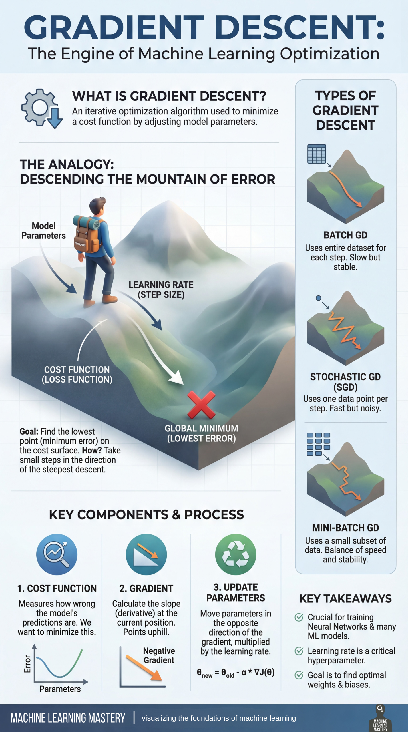
The infographic below provides a great summary of the concepts we've discussed so far, including the hill analogy, the key components, and the different types of gradient descent, which we'll touch on next.

The Mechanics of the Update Rule

Now that we have the intuition, let's look at the simple but powerful update rule that lies at the heart of gradient descent.

To summarize the key points from the article:

1. The Update Rule: At each step, every weight $w$ in the model is updated according to the rule:

   $$w_{\text{new}}=w_{\text{old}}-\alpha \cdot \frac{\partial L}{\partial w}$$

   Where:

   • $w_{\text{old}}$ is the current value of the weight.
   • $\alpha$ (alpha) is the learning rate, a small number that controls the size of our step.
   • $\frac{\partial L}{\partial w}$ is the partial derivative of the loss $L$ with respect to the weight $w$ (one component of the gradient).

2. The Learning Rate ($\alpha$): This is a critical hyperparameter.

   • If it's too small, training will be very slow as we take tiny steps.
   • If it's too large, we might overshoot the minimum and bounce around wildly, failing to converge.
   • Finding a good learning rate is a key part of training a model.

3. Types of Gradient Descent:

   • Batch Gradient Descent: Calculates the gradient using the entire dataset for each step. This is accurate but very slow on large datasets.
   • Stochastic Gradient Descent (SGD): Calculates the gradient using just one randomly chosen example per step. This is fast but the steps are "noisy" and erratic.
   • Mini-Batch Gradient Descent: The best of both worlds. It calculates the gradient using a small batch (e.g., 32, 64, 128) of examples. This is the most common approach used in practice as it balances speed and stability.

Conclusion

In this lesson, we've unpacked the fundamental mechanism of machine learning. We saw that for a model to learn, it needs a loss function to quantify its error and an optimization algorithm, gradient descent, to minimize that error.

Key Takeaways:

• A loss function measures the difference between a model's predictions and the actual values, creating a single score that the model aims to minimize.
• Gradient descent is an iterative algorithm that minimizes the loss function by repeatedly taking steps in the direction opposite to the gradient.
• The gradient is a vector of partial derivatives that points in the direction of the steepest increase in loss.
• The learning rate is a crucial hyperparameter that controls the step size in gradient descent. Choosing it correctly is vital for efficient training.
• Mini-batch gradient descent is the standard approach, offering a practical balance between the accuracy of batch GD and the speed of stochastic GD.

We now understand how a model adjusts its parameters to get "better" at a task. However, simply minimizing the loss on the training data as much as possible isn't always the best strategy. A model can become too good at fitting the training data, to the point where it fails to generalize to new, unseen data. This problem is called overfitting, and in our next lesson, we will explore what it is and discuss common techniques used to prevent it.