Overfitting and Regularization Techniques

The Problem of Overfitting

In an ideal world, a model trained on a dataset would learn the true, underlying patterns within that data. In reality, datasets contain not just patterns but also random noise and idiosyncrasies. Overfitting occurs when a model learns the training data too well, capturing both the underlying pattern and the noise. As a result, it performs exceptionally well on the data it was trained on but fails to generalize to new, unseen data. In terms of the bias-variance tradeoff we discussed earlier, an overfit model has high variance.

This divergence in performance is the classic signature of overfitting. You can see it clearly by tracking the model's loss on both the training data and a separate validation set over time.

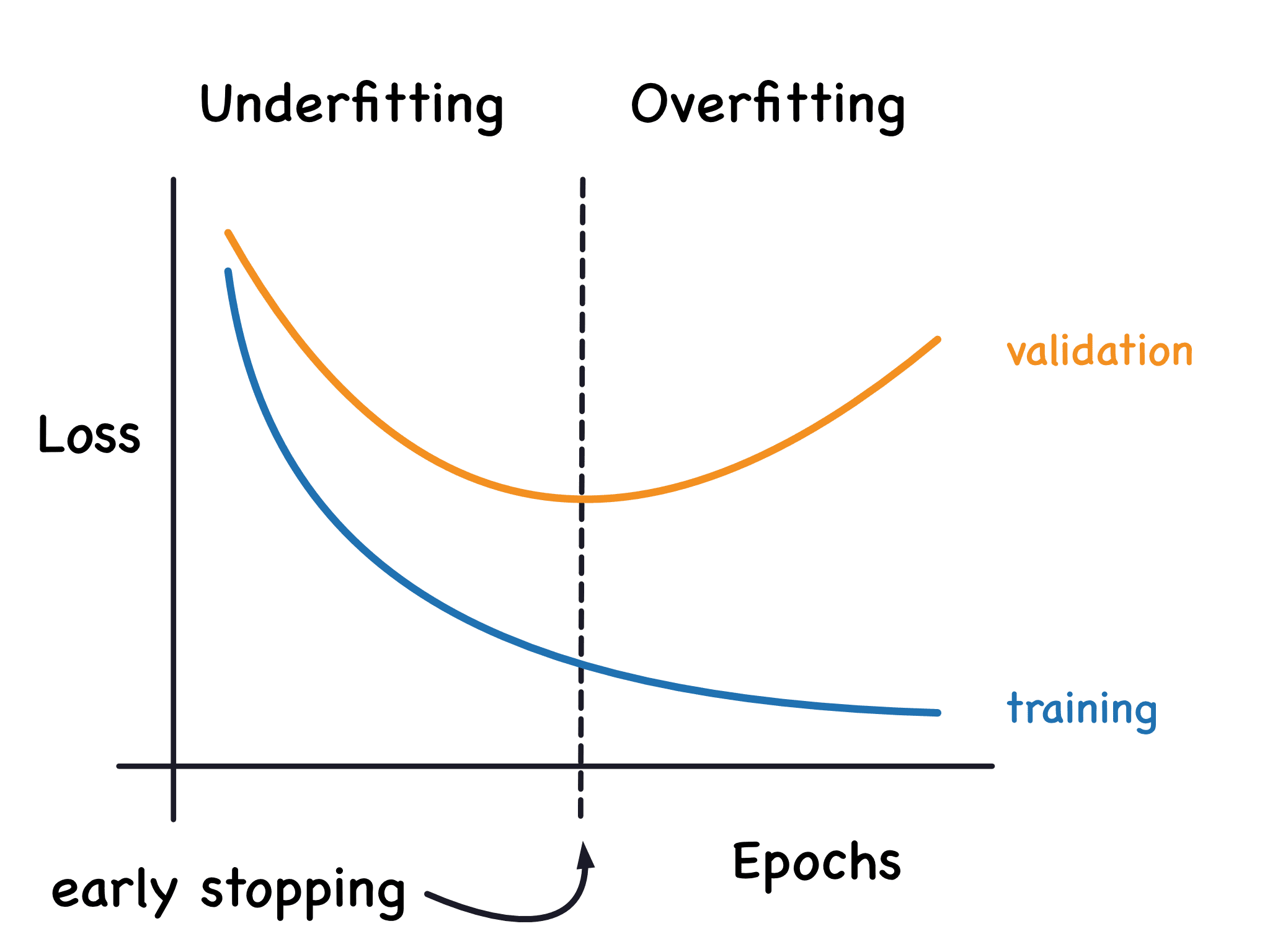
This graph illustrates the tell-tale sign of overfitting. The training loss (blue) continues to decrease as the model learns the training data more precisely. However, the validation loss (orange) decreases to a point and then begins to rise, indicating the model is losing its ability to generalize. The optimal point for training is at the bottom of the validation loss curve, and stopping there is a technique we'll discuss called "early stopping."

A model with many parameters, such as a deep neural network, is particularly susceptible to overfitting. Its high capacity gives it the "flexibility" to create a very complex decision boundary that can essentially memorize the training examples.

The following video provides a concise overview of what overfitting is and why it happens.

Overfitting isn't just a theoretical problem; it has severe consequences in production systems. A model that has memorized quirks of its training data will fail unpredictably when faced with the slightly different data distribution of the real world.

Regularization: A Strategy to Combat Overfitting

To fight overfitting, we use a set of techniques collectively known as regularization. The core idea is to constrain the model's complexity during training, making it harder for it to memorize noise. Most regularization techniques work by adding a penalty to the model's loss function. This penalty isn't for being wrong, but for being too complex.

The new, regularized loss function looks something like this:

Here, $\lambda$ (lambda) is a hyperparameter that controls the strength of the regularization. The optimization process (gradient descent) now has to find a balance: it must minimize the original loss (fit the data) while also minimizing the complexity penalty (keeping the model simple).

Let's explore the most common and effective regularization techniques you'll encounter.

Modifying the Loss Function: L1 and L2 Regularization

L1 and L2 are two of the most fundamental regularization methods. They both add a penalty based on the magnitude of the model's weights ($w$) to the loss function.

• L2 Regularization (Weight Decay or Ridge): This technique adds the sum of the squared values of all the weights to the loss function. The penalty term is $\lambda \sum w_i^2$. Because of the squaring, L2 penalizes large weights much more heavily than small ones. Its effect is to encourage all weights to shrink towards zero, resulting in a model with many small, non-zero weights. It's effective when you believe most features contribute at least a little to the final prediction.

• L1 Regularization (Lasso): This technique adds the sum of the absolute values of the weights to the loss: $\lambda \sum |w_i|$. A fascinating effect of L1 regularization is that it can force the weights of the least important features to become exactly zero. This makes it a powerful tool for automatic feature selection, resulting in a "sparse" model where only the most relevant features have non-zero weights.

The following video provides an excellent geometric intuition for why L1 leads to sparsity while L2 simply shrinks weights.

To ground this in a practical context, let's look at how to decide between L1 and L2 in a production setting.

Modifying the Network Architecture: Dropout

Dropout is a simple yet powerful regularization technique designed specifically for neural networks. During each training step, it randomly "drops out" (i.e., temporarily removes) a fraction of the neurons in a layer, along with their connections.

The intuition is that by constantly changing the network's structure, dropout prevents any single neuron from becoming overly specialized or reliant on the presence of other specific neurons. The network is forced to learn more robust and redundant representations of the data, as it can't depend on any one feature pathway being available. In effect, you are training a large ensemble of smaller, thinned networks simultaneously.

Modifying the Training Process: Early Stopping and Data Augmentation

Not all regularization techniques involve changing the loss function or network architecture. Two of the most effective methods involve modifying the training process itself.

1. Early Stopping
This is perhaps the simplest form of regularization. As we saw in the first graph, a model's performance on the validation set typically worsens after a certain point. Early stopping does exactly what its name implies: you monitor the validation loss during training and stop the process as soon as the loss stops improving and begins to increase. You then save and use the model from the epoch with the lowest validation loss. It's highly effective and requires no changes to the model or loss function, though some argue it conflates the optimization process with regularization.

2. Data Augmentation
One of the best ways to fight overfitting is to have more data. If collecting more real-world data isn't feasible, you can artificially create more through data augmentation. This involves creating new training examples by applying realistic transformations to your existing data.

• For images, this could mean flipping, rotating, cropping, or altering the brightness and contrast.
• For text, this might involve replacing words with synonyms or back-translating through another language.

The key is that the transformations must be label-preserving; a flipped image of a cat is still an image of a cat, but a flipped X-ray may no longer be medically accurate. By showing the model a wider variety of examples, data augmentation helps it learn the essential features of a class rather than superficial characteristics of specific training samples.

A Toolkit for Fighting Overfitting

These techniques—L1/L2, Dropout, Early Stopping, and Data Augmentation—form the standard toolkit for combating overfitting. The table below summarizes these and other strategies.

This table contrasts various techniques used to fight underfitting and overfitting across different aspects of the model and data.

It's important to remember a crucial point: regularization has its limits. As the following reading explains, no amount of algorithmic cleverness can compensate for fundamentally poor-quality data.

Conclusion

In this lesson, we've moved from the "how" of model training to the "how to do it well." We've seen that blindly minimizing training loss leads to overfitting, where a model fails to generalize. Regularization provides a suite of indispensable techniques to prevent this.

Key Takeaways:

• Overfitting occurs when a model learns the training data's noise and fails to generalize to unseen data. It's identified when validation loss starts to increase while training loss continues to decrease.
• Regularization is a set of techniques that penalize model complexity to prevent overfitting and improve generalization.
• L1 and L2 regularization add a penalty to the loss function based on the model's weights. L2 encourages smaller weights overall, while L1 can drive some weights to zero, performing feature selection.
• Dropout randomly deactivates neurons during training, forcing the network to learn more robust features.
• Early Stopping halts the training process when validation performance begins to degrade, effectively capturing the model at its point of optimal generalization.
• Data Augmentation artificially expands the training set, helping the model learn more general patterns.
• Ultimately, the effectiveness of regularization is capped by the quality of the training data.

Now that we have covered several core machine learning concepts, our next lesson will begin to focus more specifically on the building blocks of modern AI. We will describe the fundamental structure of a feedforward neural network, including its layers, weights, biases, and activation functions.