Feedforward Neural Network Architecture

From Pixels to Predictions: The Intuition of Neural Networks

At its core, a neural network is a computational model inspired by the brain's structure. It's designed to recognize patterns by processing information through a series of interconnected nodes, or "neurons." The simplest and most common type of architecture is the feedforward network, where information flows in only one direction—from input to output—without any loops. You can think of it as a directed acyclic graph where each node performs a simple computation.

The celebrated 3Blue1Brown video, "But what is a neural network?", provides an unparalleled visual intuition for this process. We will use it to build a mental model of how a network recognizes something complex, like a handwritten digit, by breaking the problem down into hierarchical layers of abstraction.

This idea of learning hierarchical features—from simple edges in the first hidden layer to more complex shapes in deeper layers—is a central concept in deep learning.

The Anatomy of a Neuron

Now, let's zoom in from the network level to its fundamental building block: a single neuron (or node). Each neuron in a hidden or output layer performs a two-step computation.

1. Linear Combination: It calculates a weighted sum of all its inputs and adds a bias.
2. Activation: It passes this result through a non-linear activation function.

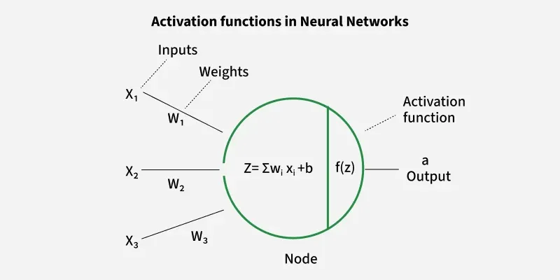
Let's break down these components:

• Weights ($w$): These are learnable parameters that determine the strength of the connection between neurons. A higher weight means the input from that connection has more influence on the neuron's output.
• Bias ($b$): This is another learnable parameter that acts like an intercept in a linear equation. It allows the neuron to shift its activation function, giving it more flexibility. A bias can be thought of as a threshold the neuron needs to overcome before it "fires" meaningfully.
• Activation Function ($f$): This is a non-linear function that determines the neuron's output. The non-linearity is crucial; without it, a multi-layer network would be mathematically equivalent to a single-layer network, unable to learn complex patterns.

This structure might seem familiar. In fact, a single neuron using a sigmoid activation function is mathematically equivalent to logistic regression, a model you may have encountered before. The Stanford lecture by Andrew Ng provides a clear bridge from logistic regression to the concept of a neuron.

Assembling the Network: Layers

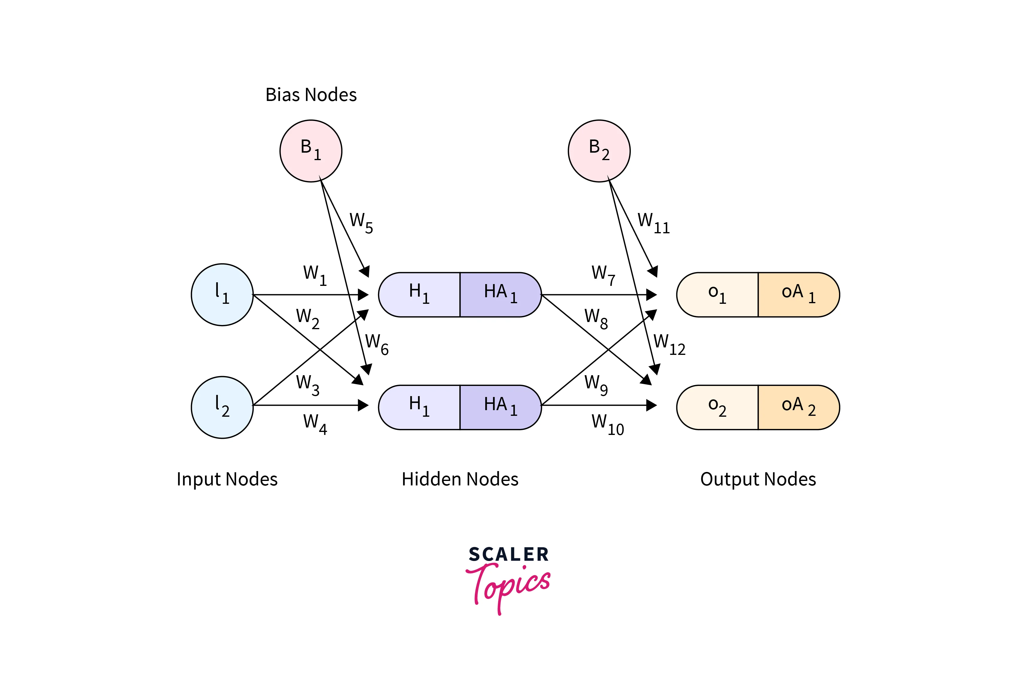
Neurons are organized into layers. A typical feedforward network, also known as a Multi-Layer Perceptron (MLP), has at least three types of layers:

1. Input Layer: This is the network's entry point. Each neuron in this layer represents a single feature of the input data (e.g., a pixel value in an image, a word embedding). This layer doesn't perform any computation; it simply passes the data to the first hidden layer.

2. Hidden Layers: These are the layers between the input and output. This is where the bulk of the computation occurs. Each neuron in a hidden layer receives inputs from all neurons in the previous layer, performs its weighted sum and activation, and passes its output to all neurons in the next layer. The "depth" of a deep learning model refers to the number of hidden layers.

3. Output Layer: This is the final layer that produces the network's prediction. Its design is specific to the task:

   • Regression: Typically a single neuron with a linear (or no) activation function to output a continuous value.
   • Binary Classification: A single neuron with a sigmoid activation function to output a probability between 0 and 1.
   • Multi-class Classification: One neuron per class, usually with a softmax activation function, which converts the raw outputs (logits) into a probability distribution where all outputs sum to 1.

The following reading from DataCamp provides a clear, structured overview of these layers and their components.

The Forward Pass: From Input to Output

The process of passing an input through the network to generate an output is called forward propagation or the forward pass. At each layer, the computations can be expressed efficiently using matrix algebra.

For a given layer $l$, the output activations $a^{(l)}$ are calculated from the previous layer's activations $a^{(l-1)}$ as follows:

1. Calculate the weighted sum plus bias, often called the pre-activation or logits, $z^{(l)}$:

   $$z^{(l)}=W^{(l)}{a}^{(l-1)}+b^{(l)}$$

2. Apply the activation function $f$ element-wise to get the new activations $a^{(l)}$:

   $$a^{(l)}=f(z^{(l)})$$

Here:

• $W^{(l)}$ is the weight matrix for layer $l$, where each column corresponds to the weights of a neuron in layer $l$.
• $b^{(l)}$ is the bias vector for layer $l$.
• $a^{(l-1)}$ is the vector of activations from the previous layer (with $a^{(0)}$ being the input data).

This process is repeated layer by layer, from the input to the output, composing functions to transform the raw data into a final prediction. The Stanford lecture explains this matrix formulation clearly.

Conclusion

In this lesson, we have dissected the architecture of a feedforward neural network. We've seen how it's built from simple, interconnected computational units called neurons, which are organized into layers.

Key Takeaways:

• Feedforward Neural Networks (FFNNs) process information in a single direction, from the input layer, through one or more hidden layers, to the output layer.
• A neuron computes a weighted sum of its inputs, adds a bias, and then applies a non-linear activation function.
• Weights and biases are the learnable parameters of the network, adjusted during training.
• Activation functions (like ReLU, Sigmoid, Softmax) introduce non-linearity, enabling the network to learn complex patterns that go beyond simple linear relationships.
• The network is structured into an input layer (receives data), hidden layers (perform computation and feature extraction), and an output layer (produces the final prediction).
• Forward propagation is the process of passing input data through the network's layers to generate a prediction, a process efficiently described by matrix operations.

Now that you understand the structure of a neural network and how it makes a prediction, the next logical question is: How does it learn? Our next lesson will introduce backpropagation, the fundamental algorithm that allows a network to calculate the error in its predictions and adjust its weights and biases accordingly.