Filtering and Measuring in Visuals

Part 1: The DAX Evaluation Engine - A 3-Stage Process

To accurately predict a measure's result, you need a mental model of how the DAX engine works. Whenever Power BI needs to display a value in a visual, it follows a consistent three-stage process for each and every cell.

1. Identify the Filter Context: The engine first looks at the cell's coordinates in the visual (e.g., the "Bikes" row, the "2022" column) and any other active filters (e.g., from slicers) to determine the complete set of filters to apply.
2. Filter the Data Model: It then applies this entire filter context to your data model. You can imagine it creating a temporary, "shrunken" version of your tables that only contains the data matching the filters.
3. Calculate the Expression: Finally, the engine executes the DAX expression of your measure, but only on this shrunken, filtered view of your data. The result is then returned to the visual.

Let's watch a video that explains and demonstrates this process perfectly.

This three-stage process is the bedrock of predicting DAX behavior.

Part 2: Deconstructing a Complex Filter Context

In a real-world report, the filter context for a single value is rarely just one filter. It's usually a combination of filters coming from multiple sources simultaneously.

Take a look at the following image. It shows a single sales value, "10.0K", and breaks down all the individual filters that combined to produce that number.

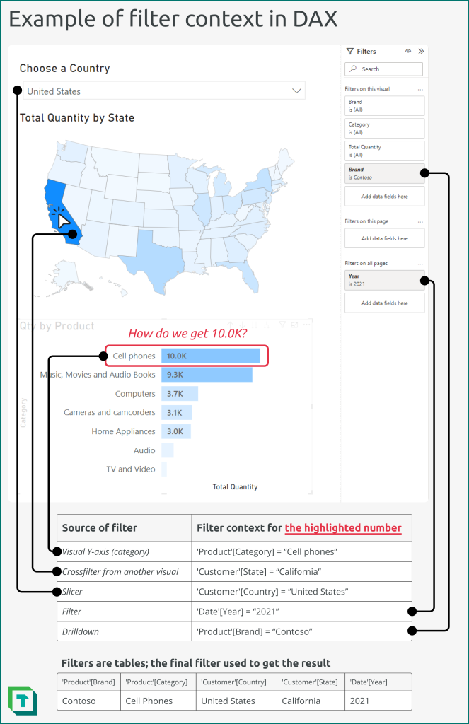
To predict a DAX result, you must first be able to identify all these contributing filters. A powerful way to conceptualize this is to think of each filter as a small table of allowed values. The total filter context is the intersection of all these small filter tables.

The following video from SQLBI provides an excellent visual representation of this idea.

Part 3: Tracing the Filter's Path Through Relationships

There's one more piece to the puzzle. As we saw last lesson, filters often start on a dimension table (like Products) but need to affect the fact table (Sales) where the calculation happens. This "travel" occurs through the relationships in your data model.

When predicting a result, you must also trace this path. A filter on Product[Category] = "Bikes" doesn't just filter the Products table; it flows along the relationship to the Sales table, ensuring that the [Total Revenue] measure only sees sales transactions for bikes.

Let's see a clear demonstration of this filter propagation.

Part 4: Your Turn - The Prediction Challenge

Now it's time to apply the "theory -> example -> application" framework. Let's use your own Power BI report to practice predicting a result.

Follow these steps in your PBIX file:

1. Set Up the Visual:

   • Go to a new, blank page in your report.
   • Create a Matrix visual.
   • Drag Product[Category] to the Rows.
   • Drag Customer[Country-Region] to the Columns.
   • Drag your [Total Revenue] measure to the Values.

2. The Challenge:

   • Look at the matrix you just created. Find the cell at the intersection of the "Bikes" category and the "United States" country-region.
   • Your task: Before looking closely at the number, try to predict it. Think through the three-stage process:
     • Stage 1: Identify Context. What are the two filters for this cell?
     • Stage 2: Filter Model. Mentally, how do these filters shrink your data? The Product table is filtered to bikes, and the Customer table is filtered to the United States. How do these filters propagate to the Sales table?
     • Stage 3: Calculate. On that doubly-filtered Sales table, what is the SUM of the Line Total column?

3. Verify Your Prediction:
   Now, let's confirm the value manually, just like in the first video. This is an invaluable skill for debugging.

   • Go to the Data view in Power BI (the grid icon on the left).
   • Select the Sales table.
   • Open the Filters pane on the right.
   • You won't see Product[Category] or Customer[Country-Region] directly, because they are in other tables. This is where relationships are key!
   • Scroll the list of filter fields until you find the fields from your related tables.
   • Under the Product table section in the filter pane, find Category. Select "Bikes".
   • Under the Customer table section, find Country-Region. Select "United States".
   • Now, look at the bottom status bar of Power BI. It will tell you the number of rows remaining in the Sales table after filtering.
   • You can't see the sum of a column here, but you have now perfectly replicated the filter context for that cell. The [Total Revenue] measure is simply summing the Line Total for these specific rows. Does the value in your matrix match what you'd expect from this filtered data?

This exercise takes you from being a passive user of DAX to an active analyst who understands what the engine is doing under the hood.

Conclusion

Great job today! You've transitioned from knowing what filter context is to understanding how it produces a result. This ability to predict outcomes is a major step forward in your DAX proficiency.

Key Takeaways:

• DAX calculates measures in a three-stage process: identify the context, filter the model, then execute the calculation.
• The filter context for a single cell is a combination of all active filters from the visual's rows, columns, slicers, and more.
• To predict a result, you must trace the filters as they propagate through relationships from dimension tables to your fact table.
• You can manually verify a filter context by using the Filters pane in the Data view to replicate the filters applied to a visual.

Preview of the Next Lesson:
Today, we focused on predicting the correct result. But what happens when Power BI gives you a strange or unexpected number? How do you figure out what went wrong? In our next lesson, we will explore why mastering evaluation context is critical for debugging DAX. You'll see how the prediction skills you learned today become your primary tool for diagnosing and fixing faulty formulas.