Revenue Forecasting with Linear Regression in Python

The Logic of Linear Trend Forecasting

At its core, forecasting with a linear trend is about finding the "line of best fit" that describes the relationship between revenue and time. We are making a simplifying assumption that revenue grows or declines by a relatively consistent amount each period. This relationship is captured by the familiar equation of a straight line:

Or, more formally, $y=mx+b$, where:

• $y$ is the dependent variable (Revenue)
• $x$ is the independent variable (Time)
• $m$ is the slope, representing the average increase in revenue per time period.
• $b$ is the y-intercept, representing the starting revenue at time zero.

The goal of our model is to analyze the historical data points and find the optimal values for the slope ($m$) and intercept ($b$) that create a line that best fits that history. We can then extend this line into the future to make our forecast.

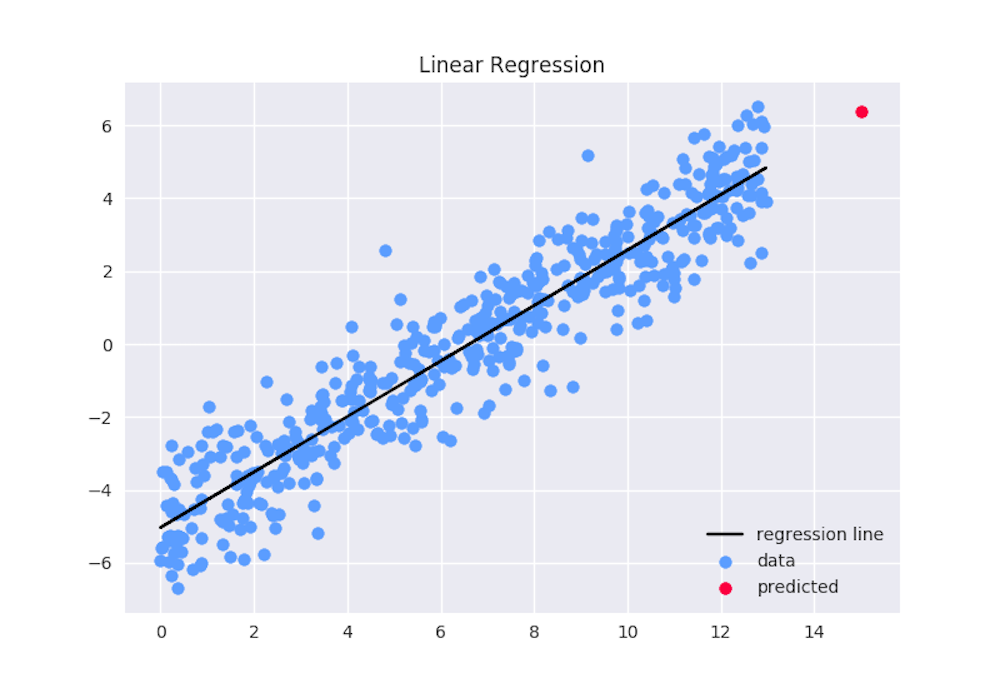
This chart illustrates the core idea. The blue dots represent historical data points (e.g., annual revenue). The black line is the linear regression line of best fit, capturing the general upward trend. The red dot is a future prediction made by extending that trend line.

Implementing a Linear Trend Forecast in Python

Let's translate this concept into a practical Python implementation. We'll use the pandas library for data handling and scikit-learn, the standard Python machine learning library, to perform the linear regression.

A fantastic article from dev.to, "A Beginner’s Guide to Time Series Forecasting Using Linear Regression," provides a very clear and straightforward code example that we can adapt for our purpose.

Step-by-Step Code Walkthrough

Let's adapt the logic from the article to forecast annual revenue for a hypothetical company.

1. Set up the environment and data
First, we import the necessary libraries and create a pandas DataFrame with our historical revenue data. Notice that we create a Time column, which is a simple integer sequence. This numerical feature is what our regression model will use as the independent variable.

import pandas as pd
import numpy as np
from sklearn.linear_model import LinearRegression
import matplotlib.pyplot as plt

# Historical revenue data (in millions)
data = {
    'Year': [2018, 2019, 2020, 2021, 2022, 2023],
    'Revenue': [100, 115, 125, 145, 150, 170]
}
df = pd.DataFrame(data)

# Create a numerical 'Time' feature for the model
df['Time'] = np.arange(len(df))

print(df)

Output:

   Year  Revenue  Time
0  2018      100     0
1  2019      115     1
2  2020      125     2
3  2021      145     3
4  2022      150     4
5  2023      170     5

2. Prepare data and fit the model
We define our independent variable X (Time) and dependent variable y (Revenue). As mentioned in the article, scikit-learn expects X to be a 2D array, so we use .values.reshape(-1, 1).

# X should be the independent variable (Time)
X = df[['Time']] # Using [['Time']] keeps it as a DataFrame
y = df['Revenue']

# Initialize and fit the linear regression model
model = LinearRegression()
model.fit(X, y)

3. Interpret the model and make predictions
Once the model is fitted, we can inspect its coef_ (the slope, $m$) and intercept_ ($b$). We can then create a set of future time periods and use model.predict() to forecast the revenue.

# The slope (m) tells us the average revenue increase per year
slope = model.coef_[0]
# The intercept (b) is the projected revenue at Time = 0
intercept = model.intercept_

print(f"Slope (Annual Growth): ${slope:,.2f} million")
print(f"Intercept (Starting Point): ${intercept:,.2f} million")

# Forecast revenue for the next 3 years (Time = 6, 7, 8)
future_time = np.array([6, 7, 8]).reshape(-1, 1)
forecasted_revenue = model.predict(future_time)

print("\nForecasted Revenue:")
for i, revenue in enumerate(forecasted_revenue, start=2024):
    print(f"Year {i}: ${revenue:,.2f} million")

Output:

Slope (Annual Growth): $13.29 million
Intercept (Starting Point): $100.33 million

Forecasted Revenue:
Year 2024: $180.06 million
Year 2025: $193.34 million
Year 2026: $206.63 million

The slope of $13.29M tells us that, on average, revenue has grown by this amount each year. This is the quantitative basis for our linear growth assumption.

4. Visualize the forecast
A plot makes the result intuitive, showing the historical data, the trend line our model found, and the future forecast.

# Plot historical data
plt.figure(figsize=(10, 6))
plt.scatter(df['Year'], df['Revenue'], label='Historical Revenue')

# Plot the regression line
plt.plot(df['Year'], model.predict(X), color='red', label='Linear Trend')

# Plot the forecasted data
future_years = [2024, 2025, 2026]
plt.scatter(future_years, forecasted_revenue, color='green', label='Forecasted Revenue')

plt.title('Revenue Forecast using Linear Trend')
plt.xlabel('Year')
plt.ylabel('Revenue (in millions)')
plt.legend()
plt.grid(True)
plt.show()

The resulting plot will look very similar in concept to the Linear Regression image we saw earlier.

Alternative Tools and Advanced Applications

While scikit-learn is a powerful and standard tool, it's worth knowing that other libraries can accomplish the same task. The NumPy library, which you've already used for array manipulation, offers a more direct function called polyfit for this kind of polynomial fitting.

The following video demonstrates how to use numpy.polyfit to model financial data. While it focuses on stock prices, the principle of regressing a value against serialized time is identical to our revenue forecasting task.

Limitations and Context

Linear trend analysis is a powerful first step, but it is crucial to understand its limitations. Your experience in business analytics will tell you that real-world growth is rarely a perfect straight line.

• It ignores seasonality: This method will not capture predictable fluctuations within a year (e.g., higher sales in Q4).
• It assumes a constant trend: It cannot model exponential growth, market saturation (S-curves), or the impact of sudden market shocks.
• It is sensitive to outliers: A single anomalous year can significantly skew the trend line.

This method is best used for stable businesses where growth is reasonably consistent or as a baseline "status quo" scenario in your financial model. More complex real-world forecasts often incorporate seasonality, cyclicality, and other drivers.

This chart shows a more complex forecast that captures seasonality (the repeating peaks and troughs) and uncertainty (the shaded confidence intervals). Our linear trend method is a simpler building block that captures the overall upward movement, but not these finer details.

Conclusion

In this lesson, you have taken a concrete step from defining assumptions to implementing them. You've learned how to quantify a historical trend and project it into the future using one of the most fundamental forecasting techniques. This process transforms a qualitative assumption ("we expect growth to continue") into a quantitative forecast that will drive our entire financial model.

Key Takeaways:

• Linear trend forecasting models revenue as a straight-line function of time, captured by the equation $y=mx+b$.
• Implementation in Python requires creating a numerical time feature (X) and using a library like scikit-learn or NumPy to fit a linear model to the historical revenue data (y).
• The model's slope ($m$) represents the average periodic growth amount and provides a quantitative basis for a growth assumption.
• This method is a foundational baseline but does not capture more complex patterns like seasonality, non-linear growth, or external shocks.

You now have the projected revenue, the top line of the Income Statement. In our next lesson, we will take this forecast and begin building the rest of our model around it. We will project a full income statement and balance sheet based on the revenue forecast and the other assumptions we've learned to develop.