Income Statement and Balance Sheet Projections

The Architecture of a Projection Model

A financial projection model is essentially a system of interconnected calculations where a few key assumptions drive the forecast for dozens of other line items. Once you have a revenue forecast, you can project many other items by assuming they will maintain a consistent relationship with sales.

For example:

• Cost of Goods Sold (COGS) is often assumed to be a certain percentage of sales (reflecting the gross margin).
• Selling, General & Administrative (SG&A) expenses might also be modeled as a percentage of sales.
• Accounts Receivable on the balance sheet will likely grow as sales grow.

The image below shows a completed three-statement model. Notice how the projections for 2019-2023 are driven by explicit assumptions like "Sales % growth," "EBITDA %," and "NWC % of Sales." Our goal today is to build the logic that creates such projections.

Projecting the Income Statement

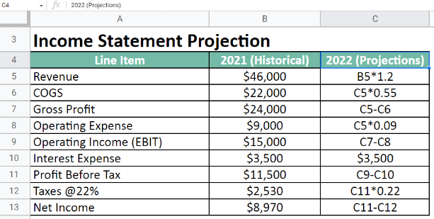
The most common method for projecting income statement line items is the "percentage of sales" method. We analyze the historical relationship between an expense and revenue, make an assumption about that relationship for the future, and apply it to our revenue forecast.

The following image from an Excel model clearly illustrates this. Revenue for 2022 is projected with a 20% growth (B5*1.2), and then COGS is projected as 55% of that new revenue number (C5*0.55).

To see a detailed walkthrough of how this is done in a spreadsheet environment, which is excellent for grasping the core concepts, the following video from Wall Street Prep is highly recommended.

Implementing Income Statement Projections in Python

Now, let's translate this logic into Python. We can represent our financial statements using pandas Series or DataFrames, which you are already familiar with. The article "Python and Finance – Power Up Your Spreadsheets" provides a superb, concise example of building a model in Python.

Let's synthesize this into a single script. We will start with a DataFrame containing historical data and our revenue forecast (as developed in the last lesson). Then, we'll define our assumptions and project the rest of the income statement.

import pandas as pd
import numpy as np




# 1. Historical Data and Revenue Forecast (from previous lesson)
years = ['2021A', '2022A', '2023A', '2024F', '2025F', '2026F']
sales_data = [150.0, 170.0, 195.0, 214.5, 236.0, 259.6] # In millions
projected_is = pd.DataFrame(index=['Sales'], columns=years)
projected_is.loc['Sales'] = sales_data




# 2. Define Assumptions
assumptions = {
    'cogs_margin': 0.60,      # COGS as 60% of Sales
    'sga_margin': 0.15,       # SG&A as 15% of Sales
    'depr_margin': 0.05,      # Depreciation as 5% of Sales
    'tax_rate': 0.22          # Tax rate of 22%
}




# 3. Project the Income Statement line items
projected_is.loc['COGS'] = projected_is.loc['Sales'] * -assumptions['cogs_margin']
projected_is.loc['Gross Profit'] = projected_is.loc['Sales'] + projected_is.loc['COGS']

projected_is.loc['SG&A'] = projected_is.loc['Sales'] * -assumptions['sga_margin']
projected_is.loc['Depreciation'] = projected_is.loc['Sales'] * -assumptions['depr_margin']




# Operating Income (EBIT) is Gross Profit minus other operating expenses
projected_is.loc['EBIT'] = projected_is.loc['Gross Profit'] + projected_is.loc['SG&A'] + projected_is.loc['Depreciation']




# For simplicity, we assume no interest expense/income for now. This will be added later.
projected_is.loc['Interest Expense'] = 0
projected_is.loc['EBT'] = projected_is.loc['EBIT'] + projected_is.loc['Interest Expense']




# Calculate tax only on positive earnings
projected_is.loc['Tax'] = projected_is.loc['EBT'].apply(lambda x: -x * assumptions['tax_rate'] if x > 0 else 0)

projected_is.loc['Net Income'] = projected_is.loc['EBT'] + projected_is.loc['Tax']

print("--- Projected Income Statement ---")
print(projected_is.round(1))

This code creates a complete projected income statement. Each line is a direct, vectorized calculation based on the sales forecast and our defined assumptions dictionary. This is a powerful and clean way to structure a model.

Projecting the Balance Sheet

Projecting the balance sheet follows a similar logic but introduces a new, critical technique: the roll-forward schedule.

1. Working Capital Items (AR, Inventory, AP):
These items are typically driven by income statement activity.

• Accounts Receivable (AR) is driven by Sales.
• Inventory is driven by COGS.
• Accounts Payable (AP) is also often driven by COGS.

2. Fixed Assets (PP&E):
Property, Plant, and Equipment does not scale directly with sales in a given year. Instead, its balance "rolls forward" based on new investments (Capital Expenditures, or Capex) and the accounting expense of depreciation. The formula is:

3. Retained Earnings:
This is the most important link between the income statement and the balance sheet. It also uses a roll-forward schedule:

The Wall Street Prep video provides an excellent conceptual explanation of these roll-forwards.

Implementing Balance Sheet Projections in Python

We can now extend our Python script to build the projected balance sheet. We will add more assumptions and implement the roll-forward logic for PP&E and Retained Earnings.

# --- Continuing from the previous script ---




# 4. Define additional assumptions for the Balance Sheet
assumptions.update({
    'ar_days': 45,            # Accounts Receivable as 45 days of sales
    'inv_days': 60,           # Inventory as 60 days of COGS
    'ap_days': 30,            # Accounts Payable as 30 days of COGS
    'capex_margin': 0.07,     # Capex as 7% of Sales
    'dividend_payout': 0.30   # Dividends as 30% of Net Income
})




# 5. Initialize and Project the Balance Sheet
# For simplicity, we'll start with some ending 2023A values
projected_bs = pd.DataFrame(columns=years)
projected_bs.loc['Accounts Receivable', '2023A'] = 25.0
projected_bs.loc['Inventory', '2023A'] = 20.0
projected_bs.loc['PP&E', '2023A'] = 100.0
projected_bs.loc['Accounts Payable', '2023A'] = 15.0
projected_bs.loc['Retained Earnings', '2023A'] = 80.0




# Project Working Capital using "days" assumptions
# Formula: (Days / 365) * Relevant Driver
projected_bs.loc['Accounts Receivable'] = (assumptions['ar_days']/365) * projected_is.loc['Sales']
projected_bs.loc['Inventory'] = (assumptions['inv_days']/365) * -projected_is.loc['COGS'] # COGS is negative
projected_bs.loc['Accounts Payable'] = (assumptions['ap_days']/365) * -projected_is.loc['COGS'] # COGS is negative




# Project PP&E using a roll-forward loop
capex = projected_is.loc['Sales'] * assumptions['capex_margin']
depreciation = -projected_is.loc['Depreciation'] # Make depreciation a positive value for subtraction

for year in range(3, len(years)): # Start from 2024F
    prev_year_col = projected_bs.columns[year - 1]
    curr_year_col = projected_bs.columns[year]
    
    beg_ppe = projected_bs.loc['PP&E', prev_year_col]
    projected_bs.loc['PP&E', curr_year_col] = beg_ppe + capex[curr_year_col] - depreciation[curr_year_col]




# Project Retained Earnings using a roll-forward loop
dividends = projected_is.loc['Net Income'] * assumptions['dividend_payout']

for year in range(3, len(years)):
    prev_year_col = projected_bs.columns[year - 1]
    curr_year_col = projected_bs.columns[year]
    
    beg_re = projected_bs.loc['Retained Earnings', prev_year_col]
    net_income = projected_is.loc['Net Income', curr_year_col]
    projected_bs.loc['Retained Earnings', curr_year_col] = beg_re + net_income - dividends[curr_year_col]


print("\n--- Projected Balance Sheet ---")
print(projected_bs.round(1))

In this script, notice how we use loops for the roll-forward accounts (PP&E and Retained Earnings). For each forecast year, we grab the ending balance from the previous year, add the inflows (Capex, Net Income), subtract the outflows (Depreciation, Dividends), and arrive at the new ending balance.

Conclusion

In this lesson, you have moved from a single-line forecast to projecting the core of a company's financial statements. We've translated a set of assumptions into multi-year projections for both the income statement and the balance sheet, implementing the fundamental logic used by financial analysts everywhere.

Key Takeaways:

• Assumption-Driven Projections: Financial models are driven by a set of explicit assumptions, such as margins (e.g., COGS as a % of Sales) or turnover days (e.g., Accounts Receivable Days).
• Percentage of Sales Method: A common and effective technique for projecting income statement items and working capital, where line items are forecast as a percentage of a driver like Sales or COGS.
• Roll-Forward Schedules: Essential for projecting balance sheet accounts like PP&E and Retained Earnings, which accumulate or decrease over time.
  • PP&E: Ending = Beginning + Capex - Depreciation
  • Retained Earnings: Ending = Beginning + Net Income - Dividends
• Linking Statements: The Retained Earnings calculation is the first major link we've built, pulling Net Income from the income statement to calculate the new balance on the balance sheet.

You now have a projected income statement and a projected balance sheet. However, they are not yet fully connected, and if you were to sum the assets and liabilities, they wouldn't balance. Why? We have ignored the cash account. In our next lesson, we will build the cash flow statement, the crucial third statement that reconciles the income statement and balance sheet, accounts for the change in cash, and ensures our entire model balances.