Hello! Welcome to your third lesson.
In our last session, we established the "what" and "why" of hydrozoning, defining it as the crucial practice of grouping plants with similar needs to improve plant health and conserve water. You learned that each hydrozone corresponds to a single irrigation valve, allowing for customized watering.
Today, we move from the concept to the practical analysis. The learning outcome for this lesson is to analyze plant water needs for lawns, shrubs, and trees to establish hydrozone boundaries. We will learn how to quantify a plant's water requirement and apply specific rules to deal with the complex, mixed plantings you'll encounter in real-world projects. This skill is the analytical foundation you need before you can draw a single line on an irrigation plan.
1. Quantifying Plant Water Needs: The Plant Factor (Kc)
As a landscape architect, you have an intuitive sense of which plants need more water. To design an efficient irrigation system, we need to translate that intuition into a number. The industry standard for this is the Crop Coefficient (Kc), also commonly called a Plant Factor (PF).
Think of Kc as a simple percentage or decimal. It represents how much water a specific plant type needs relative to a standardized reference. The basic formula for a plant's water requirement is:
We will cover Reference Evapotranspiration (), which is a measure of local climate effects, in a future lesson. For now, our entire focus is on the Crop Coefficient (Kc), which isolates the characteristics of the plant itself.
A higher Kc means a higher water need. For example:
- A lush lawn might have a Kc of 0.8.
- An established, drought-tolerant shrub might have a Kc of 0.4.
This means that under the exact same weather conditions, the lawn requires twice as much water as the shrub. This numerical difference is the primary driver for creating separate hydrozones.
To get a set of reliable, scientifically-backed Kc values for common landscape types, we will use the SLIDE (Simplified Landscape Irrigation Demand Estimation) method.
Using ANSI/ASABE S623 & SLIDE to Estimate Landscape Water Requirements
The following resource from the University of California provides a clear table of Plant Factors (the same as Kc) for broad categories of landscape plants. This approach simplifies the design process by avoiding the need to find a unique Kc value for every single plant species.
Please review 'Table 1. Plant Factors (PF) for established landscape plants...' Focus on the PF values for the plant types you will work with most: Trees, Shrubs, and different types of Turfgrass.
From this table, we can extract our core design values:
- Trees, Shrubs, Groundcovers: Kc = 0.5
- Warm-Season Turfgrass (Bermuda, Zoysia): Kc = 0.6
- Cool-Season Turfgrass (Fescue, Ryegrass): Kc = 0.8
- Annual Flowers / Bedding Plants: Kc = 0.8
This categorization is incredibly powerful. Instead of getting lost in details, you can quickly classify the major planting areas and assign them a water-use value.
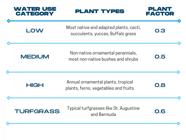
The image below provides another simplified, visual representation of this same concept.
2. The Rules for Mixed Plantings and Complex Layouts
Your goal is to design for sites with "complex plantation placements," like trees within lawns or mixed shrub-and-flower beds. This is where most beginners make mistakes. Simply knowing individual Kc values isn't enough; you must know how to combine them.
Let's return to the SLIDE resource to learn the two most important rules for handling these situations.
Using ANSI/ASABE S623 & SLIDE to Estimate Landscape Water Requirements
This reading covers the 'SLIDE Rules' and provides specific guidance on how to handle mixed plantings. It directly addresses the common, complex scenarios you will face.
Read the section 'SLIDE Rules', paying close attention to Rule #3. Then, in the following section 'Using the SLIDE Equation', find and read the two paragraphs that begin with 'Note in Table 1 the category “Mixed Plantings”...' and 'In situations where shade trees are planted within a turf area...'.
This reading gives us two non-negotiable rules for defining hydrozone boundaries:
Rule 1: The Highest Water Use Rule
When different plant types are mixed in a single hydrozone (controlled by one valve), the entire zone's water need is determined by the plant with the highest Kc value.
- Example: A planting bed contains shrubs (Kc=0.5) and annual flowers (Kc=0.8). If they are on the same irrigation valve, you must irrigate the entire zone as if it were all flowers (Kc=0.8). This means you will be consciously overwatering the shrubs to keep the flowers alive. The water-efficient solution is to separate them into two hydrozones.
Rule 2: The Tree-in-Lawn Rule
When a tree is planted within a turf area, its water demand is met by the turf irrigation schedule. You do not need a separate zone or additional water for the tree.
- Why? The turf has a higher Kc (0.6-0.8) than the tree (0.5) and is irrigated more frequently. The deep roots of the tree will easily access the water applied for the turf. Creating a separate "tree zone" in the middle of a lawn is unnecessary and complicates the system.
Test your understanding!
You are reviewing a planting plan for a villa. A large bed next to the patio includes drought-tolerant Rosemary (Kc ≈ 0.4), several Indian Hawthorn shrubs (Kc=0.5), and a cluster of high-impact Hibiscus (Kc ≈ 0.6). The client wants to keep the installation simple with a single irrigation zone for this bed.
What Kc value must you use to calculate the water needs for this entire zone? What is the consequence of this choice?
Show answer
You must use the Kc value of the highest-water-use plant, which is the Hibiscus (Kc ≈ 0.6).
The consequence is that the Rosemary and Indian Hawthorn will be consistently overwatered. While this keeps the installation simple (one valve), it wastes water and can lead to poor plant health (like root rot) for the more drought-tolerant species. The professional approach would be to recommend splitting this into at least two zones.
3. From Analysis to Action: Creating a Hydrozone Schedule
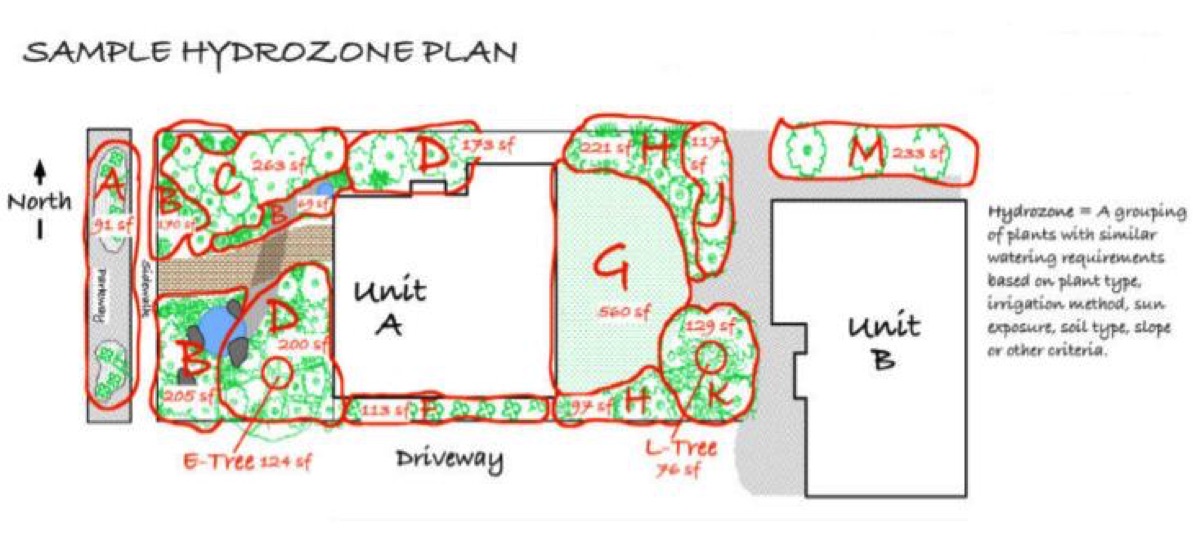
Before drawing on your site plan, it's a best practice to organize your analysis in a simple table. This helps you document your decisions and serves as a guide for zoning.
Here is a sample analysis for a hypothetical villa project:
| Location on Plan | Dominant Plant Types | Key Factor | Plant Factor (Kc) | Proposed Hydrozone |
|---|---|---|---|---|
| Front Yard | Bermuda grass lawn | Warm-Season Turf | 0.6 | Zone 1: Front Lawn |
| Back Yard | Fescue grass with oak trees | Cool-Season Turf (with trees) | 0.8 | Zone 2: Back Lawn |
| Foundation Beds | Mixed shrubs (e.g., Privet, Mock orange) | Woody Shrubs | 0.5 | Zone 3: Shrub Beds |
| Planters by Pool | Annual Flowers (e.g., Petunias) | Bedding Plants | 0.8 | Zone 4: Flower Planters |
Notice a few key decisions in this table:
- The front and back lawns are separated. Even if they were the same grass type, factors we discussed previously like sun exposure (e.g., south-facing vs. north-facing) would justify making them separate zones. Here, the different grass types (and Kc values) make it mandatory.
- The oak trees in the back lawn are handled by the "Tree-in-Lawn" rule and are included in Zone 2.
- The flowers get their own zone because their Kc (0.8) is much higher than the shrubs (0.5).
This structured analysis is the direct link between understanding the plants and defining the zones.
Conclusion
In this lesson, you've gained the analytical tools needed to properly establish hydrozone boundaries based on quantitative data, not just intuition. This is a critical step that ensures your irrigation designs are both effective for the plants and efficient with water.
Key Takeaways:
- A plant's water need is quantified by its Crop Coefficient (Kc) or Plant Factor (PF).
- For design efficiency, we use Kc values for broad plant categories (e.g., Cool-Season Turf = 0.8, Shrubs = 0.5).
- For mixed plantings in a single hydrozone, the entire zone's water need is dictated by the plant with the highest Kc.
- For trees located within a lawn, the lawn's higher water need governs the irrigation schedule; no separate zone is required for the tree.
Next Steps
You now know how to analyze the landscape. In the next lesson, "Divide a given site plan into distinct hydrozones and calculate the area (m²) of each," you will put this knowledge to work. You'll be given a site plan and a planting list, and your task will be to create the hydrozone map and then perform the area calculations needed for the next step: determining the total water volume for each zone.