Hooke's Law and Elastic Moduli

Hello! Welcome to your second lesson in the "Continuum and Fluid Mechanics" module.

In our previous lesson, we established the mathematical language to describe the state of a deformable body. We defined the stress tensor ( $σ$ ) to quantify internal forces and the strain tensor ( $ϵ$ ) to quantify local deformation. You'll recall that stress is the "cause" and strain is the "effect." Today, we will connect them.

This lesson focuses on the learning outcome: Apply Hooke's Law for linear elastic isotropic materials and use elastic moduli. We will explore the constitutive law that governs the behavior of a huge class of materials, from steel beams to rubber bands, under small deformations. This relationship, a generalization of the simple Hooke's law you've seen before, is fundamental to virtually all structural engineering and materials science.

1. Constitutive Laws: The Material's "Personality"

The relationship between stress and strain is called a constitutive law. It's not a fundamental law of physics like Newton's laws; rather, it's an empirical model that describes the behavior of a specific material. For many common materials under small deformations, this relationship is linear and elastic.

In the most general case, since stress and strain are second-rank tensors (3x3 matrices), the linear map connecting them is a fourth-rank tensor, $C_{ij k l}$ , often called the stiffness tensor:
$σ_{ij} = \sum_{k, l} C_{ij k l} ϵ_{k l}$
This tensor would have $3^{4} = 81$ components. This seems incredibly complex, but fortunately, symmetries dramatically reduce this number.

To get a sense of this complexity and its reduction, watch the first part of the following video.

Solid Mechanics Theory | Constitutive Laws (Elasticity Tensor)

This video, 'Solid Mechanics Theory | Constitutive Laws' by Dr. Clayton Pettit, gives a rigorous overview of the elasticity tensor. We'll watch a segment that shows how symmetries reduce the number of independent elastic constants.

Watch from the beginning to 10:36. Don't worry about memorizing every detail. Focus on understanding the following conceptual reductions: (0:00 - 3:19) Why a 4th-rank tensor with 81 components is needed in principle. (3:19 - 4:45) How the symmetry of the stress and strain tensors (\sigma_{ij} = \sigma_{ji}, \epsilon_{kl} = \epsilon_{lk}) reduces the number of independent constants from 81 to 36. (5:14 - 10:36) How the assumption of energy conservation in elastic materials (which implies the stiffness tensor itself is symmetric) further reduces the constants from 36 to 21. This is a crucial and often misunderstood point.

This leaves us with 21 independent elastic constants for a general linear elastic material (an anisotropic material). While important for materials like wood or single-crystal turbine blades, this is still too complex for our starting point.

2. The Isotropic Simplification: Only Two Constants Matter

Today's focus is on isotropic materials—materials whose properties are the same in all directions. Metals and many plastics, in bulk form, are excellent approximations of isotropic materials. For these materials, the 21 constants collapse to just two independent constants. All elastic behavior can be described by knowing just two numbers!

The most common pair of constants used in engineering are:

Young's Modulus (E): The measure of a material's stiffness in tension or compression.
Poisson's Ratio ( $ν$ ): A measure of the transverse contraction that occurs when a material is stretched.

Let's use these two constants to build the full 3D relationship between stress and strain.

3. Generalized Hooke's Law

Let's start from a simple case and build up, using the principle of superposition.

3.1 Normal Strains from Normal Stresses

Imagine applying only a normal stress $σ_{xx}$ to a cube of material.

The material will stretch in the x-direction. This is the simple 1D Hooke's Law: $ϵ_{xx} = \frac{σ _{xx}}{E}$ .
Due to the Poisson effect, the material will contract in the transverse directions (y and z). The strain in these directions is proportional to the axial strain: $ϵ_{y y} = ϵ_{z z} = - ν ϵ_{xx} = - ν \frac{σ _{xx}}{E}$ .

Now, what if we apply normal stresses $σ_{xx}$ , $σ_{y y}$ , and $σ_{z z}$ simultaneously? For a linear system, we can simply add the effects from each stress component.

The following video walks through this superposition argument to derive the generalized equations for normal strain.

Generalized Hooke's law

The video 'Generalized Hooke's law' by Mechanics of Materials (Libre) provides a clear, step-by-step derivation of the strain-stress relations using the principle of superposition.

Watch from 3:12 to 7:09. Follow the logic of how the total strain in one direction (e.g., \epsilon_x) is the sum of the direct strain from the stress in that direction (\sigma_x) and the Poisson-induced strains from the stresses in the other two directions (\sigma_y and \sigma_z).

As derived in the video, the resulting equations for normal strains are:

ϵ_{xx} ϵ_{y y} ϵ_{z z} = \frac{1}{E} [σ_{xx} - ν (σ_{y y} + σ_{z z})] = \frac{1}{E} [σ_{y y} - ν (σ_{xx} + σ_{z z})] = \frac{1}{E} [σ_{z z} - ν (σ_{xx} + σ_{y y})]

3.2 Shear Strains from Shear Stresses

For an isotropic material, a shear stress in one plane (e.g., $σ_{x y}$ ) only produces the corresponding shear strain ( $ϵ_{x y}$ ). There is no coupling between shear stresses and normal strains. The relationship is linear:
$σ_{x y} = G γ_{x y}$
Here, $γ_{x y}$ is the engineering shear strain, which represents the change in angle of our infinitesimal cube. It is related to our tensor shear strain by $γ_{x y} = 2 ϵ_{x y}$ . This gives:
$σ_{x y} = 2 G ϵ_{x y} or ϵ_{x y} = \frac{1}{2 G} σ_{x y}$
Similar relations hold for the yz and zx planes. The constant G is the Shear Modulus or Modulus of Rigidity, which measures a material's resistance to shearing.

Crucially, G is not an independent constant. It can be derived from E and $ν$ :
$G = \frac{E}{2 ( 1 + ν )}$

3.3 Hydrostatic Stress and the Bulk Modulus

What happens if we apply equal pressure P from all sides? This is a state of hydrostatic stress, where $σ_{xx} = σ_{y y} = σ_{z z} = - P$ , and all shear stresses are zero. The material will compress, changing its volume but not its shape.

The volumetric strain $ϵ_{V}$ is the relative change in volume, which for small strains is the trace of the strain tensor: $ϵ_{V} = \frac{Δ V}{V} \approx ϵ_{xx} + ϵ_{y y} + ϵ_{z z}$ .

The Bulk Modulus (K) measures a material's resistance to uniform compression. It is defined as:
$K = - \frac{Hydrostatic Pressure}{Volumetric Strain} = - \frac{- P}{ϵ _{V}}$

By substituting the hydrostatic stress state into our generalized Hooke's Law equations, one can show that K is also not an independent constant:
$K = \frac{E}{3 ( 1 - 2 ν )}$

The fact that $K$ must be positive for a stable material (it shouldn't expand under pressure) places a physical limit on Poisson's ratio: $ν < 0.5$ .

4. Summary of Elastic Moduli

For a linear, elastic, isotropic material, we have four key moduli. Remember, only two are independent!

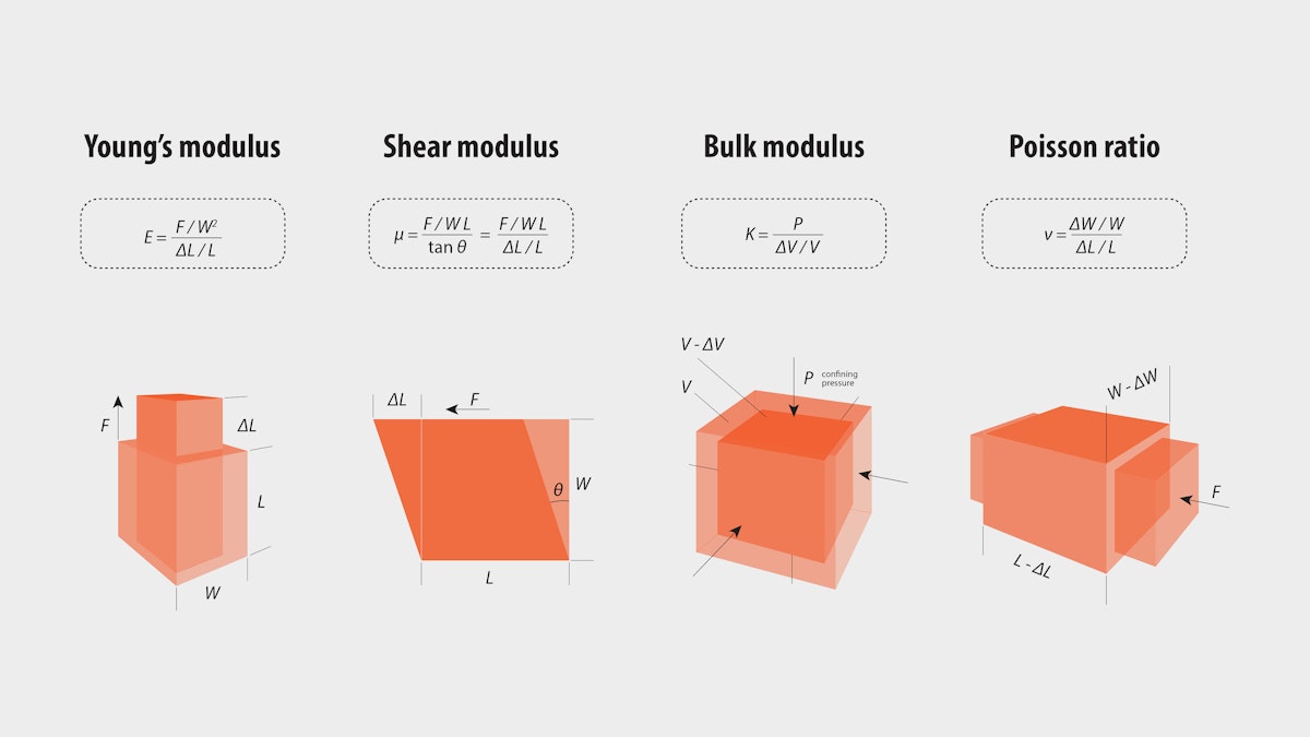
Types of Modulus of Elasticity and Poisson's Ratio — Caption: Visual representation of the four primary elastic moduli. (a) **Young's Modulus (E)** relates axial stress to axial strain. (b) **Shear Modulus (G)** relates shear stress to shear strain (angular deformation). (c) **Bulk Modulus (K)** relates hydrostatic pressure to volumetric strain. **Poisson's Ratio ($\nu$)** (not shown with its own stress state) relates the transverse strain to the axial strain in case (a).

The following document provides a concise summary and derivation of these relationships.

The usefulness of generalized Hooke's Law

The article 'The usefulness of generalized Hooke's Law' by John Maloney provides an excellent derivation and summary of the different elastic moduli.

Please read the three short sections under the heading 'The benefits'. They apply the generalized law to specific cases: 'Uniaxial stress states' to define Young's Modulus, E. 'Pure shear shear states' to define the Shear Modulus, G. 'Hydrostatic pressure states' to define the Bulk Modulus, K. Pay attention to the final formula for each modulus in terms of E and/or ( u).

Test your understanding!

A cube of steel (E = 200 GPa, $ν$ = 0.3) is subjected to a uniaxial compressive stress of $σ_{xx} = - 500$ MPa. All other stress components are zero. Calculate the three normal strain components ( $ϵ_{xx}, ϵ_{y y}, ϵ_{z z}$ ) and the Shear Modulus G.

Show answer

First, let's use the generalized Hooke's Law equations with $σ_{y y} = σ_{z z} = 0$ :

Axial Strain ( $ϵ_{xx}$ ):
$ϵ_{xx} = \frac{1}{E} [σ_{xx} - ν (0 + 0)] = \frac{σ _{xx}}{E} = \frac{- 500 \times 1 0 ^{6} Pa}{200 \times 1 0 ^{9} Pa} = - 0.0025$
This is a compressive strain of 0.25%.
Transverse Strains ( $ϵ_{y y}, ϵ_{z z}$ ):
$ϵ_{y y} = \frac{1}{E} [0 - ν (σ_{xx} + 0)] = - \frac{ν σ _{xx}}{E} = - ν ϵ_{xx} = - 0.3 \times (- 0.0025) = + 0.00075$
Since $ϵ_{z z}$ has the same form, $ϵ_{z z} = + 0.00075$ . The cube expands in the y and z directions.
Shear Modulus (G):
$G = \frac{E}{2 ( 1 + ν )} = \frac{200 GPa}{2 ( 1 + 0.3 )} = \frac{200}{2.6} \approx 76.9 GPa$

5. Tensor Formulations of Hooke's Law

Your preference for mathematical rigor will appreciate that these separate equations can be written elegantly in tensor form.

5.1 Strain from Stress (Engineering Form)

Using Einstein notation (where repeated indices are summed over) and the Kronecker delta ( $δ_{ij}$ is 1 if $i = j$ and 0 otherwise), we can write all six equations as one:
$ϵ_{ij} = \frac{1 + ν}{E} σ_{ij} - \frac{ν}{E} σ_{k k} δ_{ij}$
Here, $σ_{k k} = σ_{xx} + σ_{y y} + σ_{z z}$ is the trace of the stress tensor. Take a moment to verify that if you set $i = j = x$ , you recover the equation for $ϵ_{xx}$ , and if you set $i = x, j = y$ , you recover the equation for $ϵ_{x y}$ .

5.2 Stress from Strain (Physics Form)

It is often more fundamental to express stress as a function of strain. By inverting the relations, we arrive at a form commonly used in theoretical physics:
$σ_{ij} = 2 μ ϵ_{ij} + λ δ_{ij} ϵ_{k k}$
Here, $λ$ and $μ$ are the Lamé parameters. They are another pair of independent elastic constants.

$μ$ is exactly the same as the shear modulus, G.
$λ$ is "Lamé's first parameter".

The Lamé parameters are related to E and $ν$ by:
$λ = \frac{E ν}{( 1 + ν ) ( 1 - 2 ν )}, μ = G = \frac{E}{2 ( 1 + ν )}$
This formulation is particularly powerful as it cleanly separates the response into a shear part (proportional to $μ$ ) and a volumetric part (related to $λ$ ).

For a deep dive into this formulation and the relationships between the constants, the following text is excellent.

Linear elasticity

The textbook chapter 'Linear elasticity' by Benny Lautrup presents Hooke's law from a more fundamental physics perspective, starting with the Lamé coefficients.

Read section 11.2 'Hooke's law in isotropic materials' (pages 174-177). Focus on: The definition of Hooke's law using Lamé coefficients (\lambda, \mu), equation (11-8). The derivation of the relationships between (\lambda, \mu) and (E, ( u)), equations (11-11) through (11-13). The inverted form of Hooke's law, expressing strain in terms of stress, equation (11-18). This is the same equation we presented above in index notation.

6. Engineering Application: Plane Stress and Plane Strain

To fulfill your interest in engineering applications, let's consider two common simplifying assumptions.

Plane Stress ( $σ_{z z} = 0$ ): This applies to thin plates loaded only in the plane of the plate (e.g., the skin of an aircraft). Since the plate is thin, stress cannot develop through the thickness. We can set $σ_{z z}, σ_{x z}, σ_{y z}$ to zero in our equations, simplifying the 3D problem to a 2D one. Note that this does not mean $ϵ_{z z}$ is zero! A strain will develop through the thickness due to the Poisson effect.
Plane Strain ( $ϵ_{z z} = 0$ ): This applies to very long objects where the loading is uniform along the length (e.g., a dam or a retaining wall). Since the object can't expand or contract along its length, we can assume the strain in that direction is zero ( $ϵ_{z z} = ϵ_{x z} = ϵ_{y z} = 0$ ). This implies a non-zero stress $σ_{z z}$ must develop to prevent this strain. Again, this simplifies the problem to 2D.

These approximations are cornerstones of mechanical and civil engineering analysis, allowing for the solution of complex problems by reducing their dimensionality.

Conclusion

In this lesson, we have forged the critical link between stress and strain for the vast class of linear, elastic, and isotropic materials.

Key Takeaways:

The relationship between stress and strain is a material-dependent constitutive law.
For isotropic materials, this complex relationship simplifies dramatically and can be fully described by just two independent elastic constants.
We defined four key moduli: Young's Modulus (E), Poisson's Ratio ( $ν$ ), Shear Modulus (G), and Bulk Modulus (K).
We formulated the Generalized Hooke's Law, which can be expressed elegantly in tensor notation using either (E, $ν$ ) or the Lamé parameters ( $λ, μ$ ).

Preview of the Next Lesson:
Now that we understand how materials deform under stress, we are equipped to analyze the behavior of common structural elements. In the next lesson, we will apply these principles to a classic engineering problem: deriving and applying the equations for bending, torsion, and buckling of beams. You will see how Young's modulus and the Shear modulus directly govern how a beam bends and twists under load.

Recommended resources