Beam Mechanics: Bending, Torsion, and Buckling

1. Bending of Beams: Euler-Bernoulli Theory

Beams are structural elements designed to support loads applied transversely to their longitudinal axis. Bridges, aircraft wings, and floor joists are all examples of beams. When a beam is loaded, it deflects. To analyze this, we use the Euler-Bernoulli beam theory, which is built on a few key assumptions.

To summarize the key assumptions from the video:

1. Small deformations: The beam's deflections are small compared to its length.
2. Linear elastic isotropic material: The material obeys Hooke's law and has uniform properties in all directions.
3. Poisson's ratio effects are ignored: This is a simplification that is valid for slender beams.
4. Plane sections remain plane and normal to the longitudinal axis: This is the most critical kinematic assumption. It dictates the geometry of deformation.

Deriving the Bending Equations

The power of the "plane sections remain plane" assumption is that it allows us to derive the strain, and consequently the stress, at any point in the beam. The following video provides a rigorous derivation, and since you appreciate mathematical formalism, I encourage you to follow each step closely.

Let's summarize the results. If we let $x$ be the longitudinal axis and $y$ be the vertical deflection, and we place the origin at the centroid of the cross-section:

• The normal strain along the beam is ${ϵ}_{xx}=-y/\rho$, where $\rho$ is the local radius of curvature.
• The normal stress is ${\sigma }_{xx}=E{ϵ}_{xx}=-Ey/\rho$.
• For small deflections, $1/\rho \approx d^{2}y/d{x}^2$. This gives the flexure formula for stress:
  ${\sigma }_{xx}=-\frac{My}{I}$
  where $I={\int }_A{y}^{2}dA$ is the second moment of area of the cross-section about the neutral axis. This formula is paramount in beam design. Notice that for a given moment $M$, the stress is maximum at the points farthest from the neutral axis (largest $|y|$). This is why I-beams are so efficient: they place most of their material far from the centroid to resist bending stress effectively.

The Governing Equation for Beam Deflection

To find the deflection of a beam, we need to relate the bending moment $M$ to the applied load $q(x)$. This is done through equilibrium analysis on a differential element of the beam.

The key relationships are:
$\frac{dM}{dx}=V(x)\text{and}\frac{dV}{dx}=-q(x)$
Combining these, we get $\frac{d^{2}M}{d{x}^2}=-q(x)$.

Substituting our moment-curvature relationship $M=EI\frac{d^{2}y}{d{x}^2}$ (assuming constant flexural rigidity $EI$), we arrive at the celebrated Euler-Bernoulli beam equation:
$EI\frac{d^{4}y}{d{x}^4}=q(x)$
This fourth-order ordinary differential equation is the starting point for calculating the deflection $y(x)$ of a beam under a distributed load $q(x)$. Solving it requires four boundary conditions (e.g., specifying deflection and slope at the ends).

2. Torsion of Circular Shafts

Next, we consider torsion—the twisting of a member due to an applied torque. This is the primary mechanism for power transmission in rotating machinery like engine driveshafts and axles.

For this analysis, we will focus on shafts with a circular cross-section. This is a crucial specialization, because circular shafts under torsion behave very cleanly: their cross-sections rotate as rigid disks without distorting (warping). This is not true for non-circular shafts (e.g., square or rectangular), whose analysis is more complex.

The derivation rests on a geometric assumption analogous to the one in beam theory:

• The shear strain $\gamma$ varies linearly from the center of the shaft: $\gamma =r\frac{\varphi }{L}$, where $\varphi$ is the total angle of twist over length $L$.
• Applying Hooke's law in shear, $\tau =G\gamma$, gives the shear stress distribution: $\tau =Gr\frac{\varphi }{L}$.
• Integrating the torque produced by this stress over the cross-section yields the total torque $T$.

This process results in two fundamental equations for torsion:

1. Angle of Twist:
   $\varphi =\frac{TL}{GJ}$
2. Shear Stress:
   $\tau =\frac{Tr}{J}$
   Here, $J$ is the polar moment of inertia, a geometric property of the cross-section representing its resistance to twisting. For a solid circular shaft of radius $R$, $J=\frac{\pi }{2}{R}^4$.

Notice the beautiful analogy between the bending and torsion equations:

• Bending: Involves Moment $M$, Young's Modulus $E$, and Second Moment of Area $I$.
• Torsion: Involves Torque $T$, Shear Modulus $G$, and Polar Moment of Inertia $J$.

3. Buckling of Columns

Our final topic is buckling, a failure mode characterized by a sudden sideways deflection of a slender structural member subjected to high compressive load. Unlike yielding, which is a material failure, buckling is a failure of stability. A column can buckle even when the compressive stress is well below the material's yield strength.

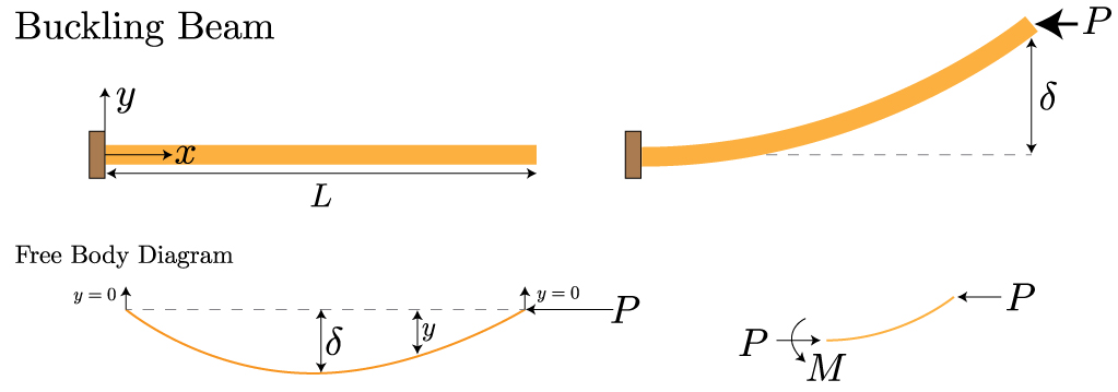
We will derive the critical buckling load for the most fundamental case: a pin-ended column, often called an Euler Column.

The derivation involves finding the load $P$ at which the column can be in equilibrium in both a straight and a slightly bent configuration. Consider the column in a slightly bent shape $y(x)$. The internal bending moment at any point $x$ is generated by the axial force $P$ acting on the moment arm $y(x)$:
$M(x)=-Py(x)$
The negative sign arises from the sign convention for bending moment (a positive deflection $y$ creates a "hogging" or negative moment).

We can now use the moment-curvature relationship we derived in the bending section, $M=EI\frac{d^{2}y}{d{x}^2}$:
$EI\frac{d^{2}y}{d{x}^2}=-Py(x)$
Rearranging gives the governing differential equation for an axially loaded column:
$\frac{d^{2}y}{d{x}^2}+\frac{P}{EI}y(x)=0$
This is a second-order linear homogeneous ODE with constant coefficients. As you know from your calculus course, this is the equation for simple harmonic motion.

To see the formal solution and the emergence of the critical load, please read the following section from a textbook on structural stability.

As the text derives, solving the ODE and applying the pin-end boundary conditions ($y(0)=0$ and $y(L)=0$) shows that a non-trivial (i.e., bent) solution only exists if:
$\sin \left(\sqrt{\frac{P}{EI}}L\right)=0$
This condition is met when $\sqrt{\frac{P}{EI}}L=n\pi$ for an integer $n=1,2,3,\dots$.

Solving for $P$ gives the possible buckling loads:
$P_n=\frac{n^2{\pi }^{2}EI}{L^2}$
The lowest load at which buckling can occur corresponds to $n=1$. This is the Euler Critical Buckling Load:
$P_{cr}=\frac{{\pi }^{2}EI}{L^2}$
This famous formula shows that the resistance to buckling depends on the material's stiffness $E$ and the beam's geometric resistance to bending $I$, and it is inversely proportional to the square of the length. This is why long, slender columns are much more susceptible to buckling.

For other boundary conditions (e.g., fixed-fixed, cantilevered), the same equation applies but with an effective length $L_e$ replacing $L$. For example, a column with two fixed ends is much more stable, having an effective length of $L_e=0.5L$, which quadruples its critical buckling load.

Conclusion

In this lesson, we have derived the foundational equations governing three critical behaviors of structural members. You've seen how the continuum mechanics principles of stress, strain, and Hooke's Law are applied to create powerful, predictive engineering models.

Key Takeaways:

• Bending: Governed by the Euler-Bernoulli equation $EI{y}^{\prime \prime \prime \prime }=q(x)$. Bending stress is given by $\sigma =-My/I$. Resistance is dictated by the flexural rigidity, $EI$.
• Torsion: For circular shafts, the angle of twist is $\varphi =TL/GJ$, and shear stress is $\tau =Tr/J$. Resistance is dictated by the torsional rigidity, $GJ$.
• Buckling: A stability failure for slender columns. The critical compressive load for a pin-ended column is $P_{cr}={\pi }^{2}EI/L^2$, again depending on the flexural rigidity $EI$.

Preview of the Next Lesson:
We have now completed our initial foray into solid mechanics. In the next lesson, we will pivot to the second major theme of this module: fluid mechanics. We will begin by deriving one of the most fundamental principles in fluid dynamics: the continuity equation, which is an expression of the conservation of mass for a fluid flow.