Laminar Pipe Flow and Reynolds Number

1. The Character of Flow: Laminar vs. Turbulent

When a fluid flows through a pipe, its motion isn't always smooth and orderly. Depending on factors like speed, pipe size, and fluid properties, the flow can be either smooth and layered (laminar) or chaotic and swirling (turbulent).

The distinction between these regimes is not just academic; it dramatically affects properties like pressure drop and heat transfer. The key question is: what determines whether a flow is laminar or turbulent? The answer lies in the competition between inertia, which tends to cause instability and chaos, and viscosity, which tends to dampen disturbances and maintain order.

2. The Reynolds Number: A Measure of Flow Regime

To quantify this balance, physicists and engineers use a dimensionless quantity called the Reynolds number ($Re$). It is defined as the ratio of inertial forces to viscous forces.

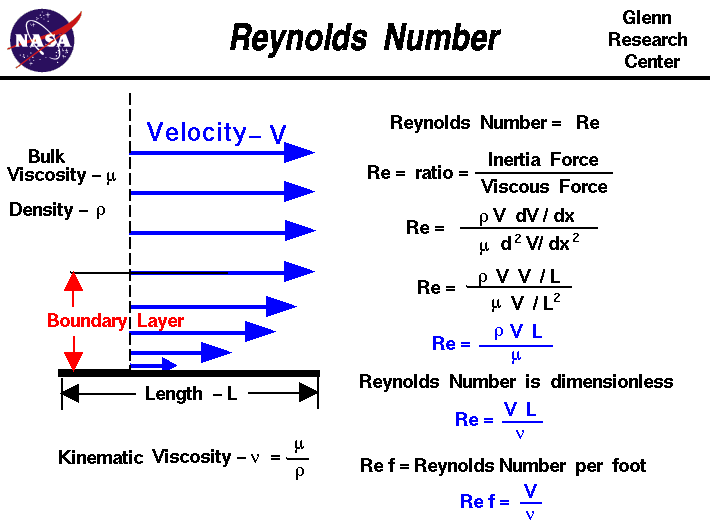
For flow in a pipe, the Reynolds number is given by:
$R{e}_D=\frac{\text{Inertial Forces}}{\text{Viscous Forces}}=\frac{\rho \bar{u}D}{\mu }=\frac{\bar{u}D}{\nu }$
where:

• $\rho$ is the fluid density.
• $\bar{u}$ is the average velocity of the flow.
• $D$ is the pipe diameter.
• $\mu$ is the dynamic viscosity.
• $\nu =\mu /\rho$ is the kinematic viscosity.

Experiments have established critical values for $R{e}_D$ that define the flow regimes in a pipe. The following video introduces these values and reinforces the concept.

As the video explains, the accepted ranges are:

• $R{e}_D\lesssim 2300$: Laminar flow. Viscous forces dominate, and the flow is smooth and predictable.
• $2300\lesssim R{e}_D\lesssim 4000$: Transitional flow. The flow is unstable and can switch between laminar and turbulent characteristics.
• $R{e}_D\gtrsim 4000$: Turbulent flow. Inertial forces dominate, leading to chaotic, unpredictable motion.

Our focus for today's analytical solution is squarely on the laminar regime.

3. Solving Navier-Stokes for Pipe Flow: Hagen-Poiseuille Flow

We now have the tools to solve a classic problem: finding the exact velocity profile for a steady, laminar flow through a long, straight, circular pipe. This is known as Hagen-Poiseuille flow.

The derivation involves applying the Navier-Stokes and continuity equations in cylindrical coordinates ($r,\theta ,z$) and simplifying them based on a set of reasonable assumptions.

The Fluid Matters channel provides an excellent, rigorous derivation that we will follow.

Summary of the Derivation

Let's recap the mathematical steps from the video. We start with the incompressible Navier-Stokes equation in the axial ($z$) direction in cylindrical coordinates:
$\rho \left(\frac{\partial u_z}{\partial t}+u_r\frac{\partial u_z}{\partial r}+\frac{u_{\theta }}{r}\frac{\partial u_z}{\partial \theta }+u_z\frac{\partial u_z}{\partial z}\right)=-\frac{\partial p}{\partial z}+\mu \left[\frac{1}{r}\frac{\partial }{\partial r}\left(r\frac{\partial u_z}{\partial r}\right)+\frac{1}{r^2}\frac{{\partial }^2{u}_z}{\partial {\theta }^2}+\frac{{\partial }^2{u}_z}{\partial z^2}\right]+\rho g_z$
Applying the assumptions (steady, fully developed, no swirl, axi-symmetric, horizontal pipe) simplifies this dramatically to:
$0=-\frac{dp}{dz}+\mu \frac{1}{r}\frac{d}{dr}\left(r\frac{d{u}_z}{dr}\right)$
Rearranging gives us the key ODE:
$\frac{d}{dr}\left(r\frac{d{u}_z}{dr}\right)=\frac{r}{\mu }\frac{dp}{dz}$
Integrating this twice and applying the boundary conditions ($u_z(R)=0$ and $d{u}_z/dr{|}_{r=0}=0$) yields the celebrated parabolic velocity profile:
$u_z(r)=\frac{R^2}{4\mu }\left(-\frac{dp}{dz}\right)\left(1-\frac{r^2}{R^2}\right)$
The velocity is maximum at the centerline ($r=0$) and zero at the wall ($r=R$). The term $-dp/dz$ is the pressure gradient driving the flow; it must be positive for flow in the +z direction (i.e., pressure must drop).

4. Volumetric Flow Rate and Poiseuille's Law

From an engineering perspective, we are often most interested in the total volume of fluid passing through the pipe per unit time, the volumetric flow rate $Q$. We find this by integrating the velocity profile over the pipe's cross-sectional area.

The integration is:
$Q={\int }_0^R{u}_z(r)(2\pi r)dr={\int }_0^R\frac{1}{4\mu }\left(-\frac{dp}{dz}\right)(R^2-r^2)(2\pi r)dr$
Solving this definite integral gives Poiseuille's Law:
$Q=\frac{\pi R^4}{8\mu }\left(-\frac{dp}{dz}\right)=\frac{\pi D^4}{128\mu }\frac{\Delta p}{L}$
where we've substituted $R=D/2$ and recognized that for a fully developed flow, the constant pressure gradient $-dp/dz$ can be written as the total pressure drop $\Delta p$ over a pipe length $L$.

This is a remarkable result. It shows that for laminar flow, the flow rate is proportional to the pressure drop and, most strikingly, to the fourth power of the pipe's radius (or diameter).

5. Application and Verification

We now have a complete model for laminar pipe flow. Let's see it in action with a numerical example that ties everything together. We will calculate the flow rate using Poiseuille's Law and then compute the Reynolds number to verify that our initial assumption of laminar flow was valid.

This example perfectly illustrates the standard engineering workflow: assume a flow regime (laminar), perform calculations based on that assumption, and then verify the assumption. If the Reynolds number had been > 2300, our Poiseuille's Law calculation would be invalid, and a different model for turbulent flow would be needed.

For a consolidated written summary of this entire derivation, from the initial assumptions to Poiseuille's Law and the Reynolds number condition, you can refer to the following notes.

Conclusion

In this lesson, we moved from the abstract formulation of the Navier-Stokes equations to a concrete, analytical solution for a problem of immense practical importance. We derived the parabolic velocity profile for laminar flow in a pipe and the resulting Poiseuille's Law, which quantifies the flow rate.

Key Takeaways:

• The Reynolds number ($R{e}_D=\rho \bar{u}D/\mu$) is a crucial dimensionless parameter that determines whether a pipe flow is laminar ($R{e}_D\lesssim 2300$) or turbulent.
• For laminar flow, the Navier-Stokes equations can be solved to yield a parabolic velocity profile, with maximum velocity at the center and zero at the walls.
• Poiseuille's Law ($Q\propto \Delta p{D}^4/\mu L$) shows that the flow rate is highly sensitive to the pipe's diameter.
• The process of solving fluid dynamics problems often involves assuming a flow regime, calculating the flow properties, and then verifying the initial assumption with the Reynolds number.

Preview of the Next Lesson:
We will now shift our focus within continuum mechanics from fluids back to solids. In the next lesson, we will "Apply Hooke's Law for linear elastic isotropic materials and use elastic moduli." We will explore how solid materials deform under applied forces, introducing fundamental concepts like stress, strain, and the material properties that connect them, laying the groundwork for analyzing the mechanics of structures and materials.