Navier-Stokes Equations for Newtonian Fluids

1. The Challenge of Real Fluids: Closing the Equations

Recall the momentum equation in its general form, which states that the mass times acceleration of a fluid element equals the sum of forces acting on it:
$\rho \frac{D\vec{u}}{Dt}=\nabla \cdot \mathbf{\sigma }+\rho \vec{g}$
Here, $\rho \frac{D\vec{u}}{Dt}$ is the mass times acceleration per unit volume (with $\frac{D}{Dt}$ being the material derivative), $\rho \vec{g}$ represents body forces like gravity, and $\mathbf{\sigma }$ is the stress tensor, which describes all the surface forces.

In our last lesson on ideal fluids, we made the simple assumption that the only surface force is isotropic pressure, so $\mathbf{\sigma }=-p\mathbf{I}$. This led to Euler's equation. However, this model is incomplete. It doesn't account for friction. This leads to a fundamental problem: we have more unknowns (velocities, pressure, and now stresses) than we have equations (mass and momentum conservation). We need a way to relate the stresses to the fluid motion itself.

This video from MIT provides an excellent overview of why this "closure problem" exists and how we begin to solve it.

As the video explained, our task is to find a constitutive equation that defines the viscous stress tensor (often called the deviatoric stress) in terms of the velocity field.

2. The Foundation: Newton's Law of Viscosity

For many common fluids like air and water, the relationship between stress and deformation rate is linear. These are called Newtonian fluids. The simplest case is a 1D shear flow.

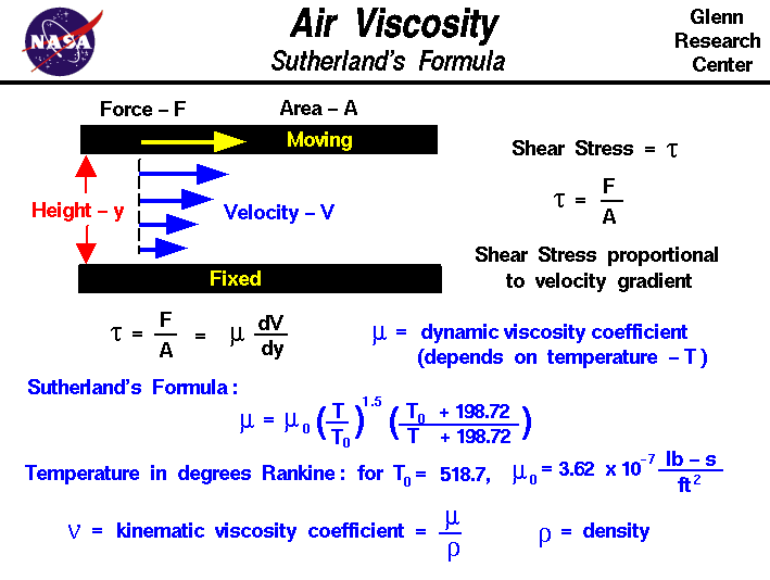
The 1D relationship is $\tau =\mu \frac{du}{dy}$. Our goal is to generalize this to a full 3D tensor equation relating the viscous stress tensor $\mathbf{\tau }$ to the velocity gradient tensor $\nabla \vec{u}$.

3. The Full Derivation: From Momentum Conservation to the Final Equation

We will now walk through the complete derivation. The following video provides a clear, step-by-step construction of the Navier-Stokes equations from a control volume perspective, which is a standard approach in engineering. We will use it as our guide, pausing to bring in more rigorous mathematical arguments where necessary.

The video brings us to a crucial point. We have a set of momentum equations, but they involve the unknown components of the stress tensor ${\tau }_{ij}$. As the video asks, "Is there a relationship between stresses $\tau$ and velocity components $u,v,w$?". Yes, and this is where the physics of the fluid comes in.

3.1. The Constitutive Relation for a Newtonian Fluid (A Deeper Dive)

To establish this relationship rigorously, we rely on a few key assumptions about the fluid:

1. Homogeneity: The relationship between stress and deformation rate is the same at all points in the fluid.
2. Isotropy: The fluid has no preferred direction. The relationship is independent of the coordinate system's orientation.
3. Linearity: The viscous stresses are a linear function of the rate of fluid deformation (the Newtonian fluid assumption).

Under these assumptions, we can derive the most general possible form for the viscous stress tensor. A key insight from physics is that for an isotropic fluid, the viscous stress can only depend on the part of the motion that causes deformation (stretching and shearing), not pure rotation. The velocity gradient tensor, $\nabla \vec{u}$, can be decomposed into a symmetric part (the rate-of-strain tensor, $\mathbf{E}$) and an anti-symmetric part (the vorticity tensor, $\mathbf{\Omega }$). The viscous stress depends only on the symmetric part, $\mathbf{E}$.

This next reading from a graduate-level fluid dynamics course provides the formal derivation of this constitutive law. This is a mathematically dense but essential piece of the argument.

The key result from that rigorous derivation is the constitutive equation for a general Newtonian fluid:
$\mathbf{\tau }=2\mu \mathbf{E}+\lambda (\text{tr}(\mathbf{E}))\mathbf{I}$
where:

• $\mathbf{E}=\frac{1}{2}(\nabla \vec{u}+(\nabla \vec{u}{)}^T)$ is the rate-of-strain tensor.
• $\text{tr}(\mathbf{E})=\nabla \cdot \vec{u}$ is the divergence of the velocity, representing the rate of volume expansion.
• $\mu$ is the familiar dynamic viscosity (related to shear deformation).
• $\lambda$ is the second coefficient of viscosity (related to volumetric deformation).

3.2. Stokes' Hypothesis and Final Assembly

We now have an expression for the stress tensor, but it involves two viscosity coefficients. George Stokes proposed a simplifying assumption known as Stokes' hypothesis. It relates $\lambda$ and $\mu$ by assuming that the mechanical pressure (the average of the normal stresses) is equal to the thermodynamic pressure. This leads to the relation:
$\lambda =-\frac{2}{3}\mu$

With this final piece, we have a complete model for the stress tensor in terms of velocity gradients. Now we can substitute it back into the Cauchy momentum equation to get our final result.

Let's return to the video to see the final steps of the derivation.

For a more detailed written explanation of this final assembly, you can refer to the article "How to Derive the Navier-Stokes Equations" by CFD.University, specifically the sections "Finding a constitutive equation for the shear stresses" through "Putting it all together: the final Navier-Stokes momentum equation".

4. The Navier-Stokes Equations

Let's write down the final results clearly.

Compressible Form

By substituting $\mathbf{\sigma }=-p\mathbf{I}+2\mu \mathbf{E}-\frac{2}{3}\mu (\nabla \cdot \vec{u})\mathbf{I}$ into the Cauchy momentum equation and expanding the material derivative, we get the compressible Navier-Stokes equation:

$\underset{\text{Inertia (Mass x Acceleration)}}{\underbrace{\rho \left(\frac{\partial \vec{u}}{\partial t}+(\vec{u}\cdot \nabla )\vec{u}\right)}}=\underset{\text{Pressure Force}}{\underbrace{-\nabla p}}+\underset{\text{Viscous Force}}{\underbrace{\mu {\nabla }^2\vec{u}+\frac{1}{3}\mu \nabla (\nabla \cdot \vec{u})}}+\underset{\text{Body Force}}{\underbrace{\rho \vec{g}}}$

This is a very general and complex equation that describes flows where density can change, such as in high-speed aerodynamics or acoustics.

Incompressible Form

For a vast range of engineering applications (including most liquid flows and low-speed gas flows), we can assume the fluid is incompressible. This simplifies things immensely. The continuity equation becomes:
$\nabla \cdot \vec{u}=0$
When we substitute this into the compressible Navier-Stokes equation, the term involving $\nabla (\nabla \cdot \vec{u})$ vanishes. This leaves us with the much more common incompressible Navier-Stokes equation:

$\rho \left(\frac{\partial \vec{u}}{\partial t}+(\vec{u}\cdot \nabla )\vec{u}\right)=-\nabla p+\mu {\nabla }^2\vec{u}+\rho \vec{g}$

This vector equation, combined with the incompressible continuity equation ($\nabla \cdot \vec{u}=0$), forms a closed system of four partial differential equations for the four unknowns: the three velocity components ($u,v,w$) and the pressure $p$.

Conclusion

Today, we have made the significant leap from ideal fluids to real, viscous fluids. The derivation of the Navier-Stokes equations is a landmark achievement in classical physics, providing the fundamental basis for the entire field of fluid dynamics.

Key Takeaways:

• The Navier-Stokes equations are the expression of Newton's second law ($F=ma$) applied to a viscous fluid element.
• The derivation requires a constitutive relation to model the internal frictional forces. For a Newtonian fluid, we assume the viscous stress is linearly proportional to the local rate of strain.
• The full compressible equation is complex, but for many practical cases, the flow is assumed incompressible ($\nabla \cdot \vec{u}=0$), leading to a simpler, widely used form of the equations.
• The final equation balances inertial forces against pressure, viscous, and body forces.

Preview of the Next Lesson:
Deriving these equations is one thing; solving them is another. They are notoriously difficult nonlinear partial differential equations. In our next lesson, "Analyze laminar flow in pipes (Poiseuille flow) and characterize flow regimes using the Reynolds number," we will take on one of the few cases where the Navier-Stokes equations can be solved analytically. We will apply the equations in cylindrical coordinates to solve for the velocity profile of fluid flowing through a circular pipe, a classic problem with immense engineering importance.