From Lagrangian to Hamiltonian: Deriving Hamilton's Equations

1. The Legendre Transformation: The Mathematical Tool

At its heart, a Legendre transformation is a systematic way to change the independent variable of a function. Instead of describing a function $y(x)$ by its value at each point $x$, we can describe it by the slope of its tangent line, $P=dy/dx$, at each point. The Legendre transform, $\Psi (P)$, is the new function that contains all the original information, but expressed in terms of the slope $P$.

The transformation is defined by the relationship between the original function and the y-intercept of its tangent lines.

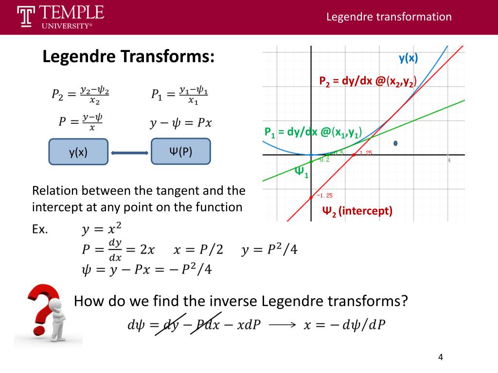
To formalize this and see its properties, let's watch a detailed explanation.

A key condition for the Legendre transformation to be well-defined is that the relationship between the old variable and the new one (e.g., between $u$ and $v=\partial f/\partial u$) must be invertible. For a function $f(u)$, this corresponds to the function being either strictly convex or strictly concave, ensuring that each slope $v$ corresponds to a unique point $u$.

2. From the Lagrangian to the Hamiltonian

Now, let's apply this mathematical tool to our physical system. The Lagrangian, $L$, is a function of generalized coordinates and velocities: $L(q_i,{\dot{q}}_i,t)$. Our goal is to create a new function, the Hamiltonian $H$, that depends on coordinates and momenta: $H(q_i,p_i,t)$.

This is a perfect scenario for a Legendre transformation. We will transform the Lagrangian with respect to the generalized velocities ${\dot{q}}_i$.

• The original function is the Lagrangian: $L(q_i,{\dot{q}}_i,t)$.
• The variables we transform are the generalized velocities ${\dot{q}}_i$. These are the "active" variables.
• The generalized coordinates $q_i$ and time $t$ are held constant during the transformation. These are the "passive" variables.
• The new variables are the generalized momenta $p_i$, defined as the partial derivatives of the Lagrangian with respect to the active variables:
  $p_i=\frac{\partial L}{\partial {\dot{q}}_i}$
• The new function is the Hamiltonian $H$, which is the Legendre transform of $L$:
  $H={\sum }_i{p}_i{\dot{q}}_i-L$

Let's see how this mapping works in detail.

So, the Hamiltonian is formally defined as:

A crucial and often tricky step follows this definition. The final expression for the Hamiltonian must be a function of only $q_i,p_i$, and $t$. To achieve this, you must first calculate $p_i=\partial L/\partial {\dot{q}}_i$, and then algebraically solve these equations to express each ${\dot{q}}_i$ in terms of the $p_i$ and $q_i$. These expressions for ${\dot{q}}_i$ are then substituted back into the definition of $H$.

This is a common source of error. The following resource highlights why this step is so critical.

3. Deriving Hamilton's Equations of Motion

Now that we have the Hamiltonian $H(q,p,t)$, how do we find the equations of motion? We need to derive Hamilton's canonical equations. The derivation is a beautiful piece of calculus that flows from the definition of $H$.

Let's start by taking the total differential of the Hamiltonian, $H(q,p,t)$. (For simplicity, we'll write it for one degree of freedom, but it generalizes with a sum over the index $i$).
$dH=\frac{\partial H}{\partial q}dq+\frac{\partial H}{\partial p}dp+\frac{\partial H}{\partial t}dt$
This simply follows from the chain rule for a function of three variables.

Next, we take the differential of the definition of the Hamiltonian, $H=p\dot{q}-L(q,\dot{q},t)$:
$dH=(dp)\dot{q}+p(d\dot{q})-dL$
We know from the chain rule that $dL=\frac{\partial L}{\partial q}dq+\frac{\partial L}{\partial \dot{q}}d\dot{q}+\frac{\partial L}{\partial t}dt$. Substituting this in:
$dH=\dot{q}dp+pd\dot{q}-\left(\frac{\partial L}{\partial q}dq+\frac{\partial L}{\partial \dot{q}}d\dot{q}+\frac{\partial L}{\partial t}dt\right)$
Now we use two key relationships from the Lagrangian formalism:

1. The definition of generalized momentum: $p=\frac{\partial L}{\partial \dot{q}}$
2. The Euler-Lagrange equation: $\frac{\partial L}{\partial q}=\frac{d}{dt}\left(\frac{\partial L}{\partial \dot{q}}\right)=\dot{p}$

Substituting these into our expression for $dH$:
$dH=\dot{q}dp+pd\dot{q}-\left(\dot{p}dq+pd\dot{q}+\frac{\partial L}{\partial t}dt\right)$
The terms $pd\dot{q}$ cancel out, leaving a remarkably clean expression:
$dH=\dot{q}dp-\dot{p}dq-\frac{\partial L}{\partial t}dt$
Now we compare our two expressions for $dH$. By matching the coefficients of the independent differentials $dq$, $dp$, and $dt$, we arrive at Hamilton's equations:

These are Hamilton's canonical equations of motion. Notice their beautiful symmetry (apart from the minus sign). Instead of one second-order differential equation from Lagrange, we now have two first-order differential equations.

For a more guided walk-through of this derivation, we can use our primary resources.

4. Worked Example: The Simple Harmonic Oscillator

Let's solidify this entire process with a concrete example: the one-dimensional simple harmonic oscillator.

The Lagrangian is $L=T-V=\frac{1}{2}m{\dot{q}}^2-\frac{1}{2}k{q}^2$.

1. Find the momentum $p$:
   $p=\frac{\partial L}{\partial \dot{q}}=m\dot{q}$

2. Invert to find $\dot{q}(p)$:
   $\dot{q}=\frac{p}{m}$

3. Construct the Hamiltonian $H(q,p)$:
   $H=p\dot{q}-L=p\left(\frac{p}{m}\right)-\left(\frac{1}{2}m{\left(\frac{p}{m}\right)}^2-\frac{1}{2}k{q}^2\right)=\frac{p^2}{2m}+\frac{1}{2}k{q}^2$
   As we found earlier, $H$ is the total energy, $T+V$.

4. Write and solve Hamilton's equations:

   • $\dot{q}=\frac{\partial H}{\partial p}=\frac{\partial }{\partial p}\left(\frac{p^2}{2m}+\frac{1}{2}k{q}^2\right)=\frac{p}{m}$
   • $\dot{p}=-\frac{\partial H}{\partial q}=-\frac{\partial }{\partial q}\left(\frac{p^2}{2m}+\frac{1}{2}k{q}^2\right)=-kq$

We now have two coupled, first-order ODEs. The first tells us $\dot{q}=p/m$, which is just the definition of momentum. Differentiating it gives $\ddot{q}=\dot{p}/m$. Substituting the second equation ($\dot{p}=-kq$) into this gives:
$\ddot{q}=\frac{-kq}{m}⟹m\ddot{q}+kq=0$
This is exactly the familiar second-order equation of motion for a simple harmonic oscillator we would get from Newton's second law or the Euler-Lagrange equation.

The following video segment walks through this exact example.

Conclusion

In this lesson, we have built the foundation for an entirely new formulation of classical mechanics. We've seen that the Hamiltonian formalism provides a symmetric and powerful description of dynamics in phase space.

Key Takeaways:

• Hamiltonian mechanics describes a system in phase space using generalized coordinates $q$ and generalized momenta $p$.
• The Hamiltonian $H(q,p,t)$ is obtained from the Lagrangian $L(q,\dot{q},t)$ via a Legendre transformation with respect to the generalized velocities $\dot{q}$.
• The definition is $H=\sum p_i{\dot{q}}_i-L$, where $p_i=\partial L/\partial {\dot{q}}_i$, and all ${\dot{q}}_i$ must be eliminated in favor of $p_i$.
• The dynamics of the system are governed by Hamilton's canonical equations, a set of $2n$ first-order ODEs:
  ${\dot{q}}_i=\frac{\partial H}{\partial p_i}\text{and}{\dot{p}}_i=-\frac{\partial H}{\partial q_i}$

Preview of the Next Lesson:
We have successfully derived the machinery of the Hamiltonian formalism. In our next lesson, we will put it to use. We will focus on solving mechanics problems using the Hamiltonian formalism, applying these techniques to more complex systems and exploring the unique insights and advantages this powerful framework offers.